Business StatisticsUnit 27 min read

Measures of Central Tendency and Dispersion – Key Concepts

Unit 2 of Business Statistics: introduces mean, median, mode, range, variance, standard deviation, inter‑quartile range, coefficient of variation, and their calculation, interpretation, and application in business contexts.

Padhai · Based on the official syllabus and past papers
Updated 3 Oct 2026

Key points

Mean is the arithmetic average, sensitive to extreme values.
Median is the middle value, robust against outliers.
Mode identifies the most frequent observation.
Range, variance, and standard deviation quantify spread; IQR is a robust measure of dispersion.
Coefficient of variation allows comparison of variability across different units or scales.
Choosing the right measure depends on data shape, presence of outliers, and business question.

Measures of Central Tendency

Central tendency summarizes a data set by a single representative value.

Measure	Formula	When to Use	Example
Mean	$\overset{x}{ˉ} = \frac{1}{n} \sum_{i = 1}^{n} x_{i}$	Symmetric data, no extreme outliers	Average monthly sales
Median	Middle value after ordering	Skewed data, outliers	Median household income
Mode	Most frequent value	Categorical or discrete data	Most common product category

Worked Example – Monthly Income Distribution

Income (Rs.)	Families
<100	5
100–199	10
200–299	5
300–399	10
400–499	9

Assume each family in a band has the midpoint value of that band.
$\overset{x}{ˉ} = \frac{5 ( 50 ) + 10 ( 150 ) + 5 ( 250 ) + 10 ( 350 ) + 9 ( 450 )}{5 + 10 + 5 + 10 + 9} = \frac{250 + 1500 + 1250 + 3500 + 4050}{39} = \frac{11550}{39} \approx 296.15 Rs$

Median: 39 families → 20th and 21st values after ordering.
The 20th falls in 300–399 band, 21st also in 300–399 → median ≈ 350 Rs.

Mode: 100–199 and 300–399 bands both have 10 families → two modes (bimodal).

Choosing the measure: The distribution is slightly right‑skewed (long tail above 400). Median is more robust, so for reporting average income we recommend the median (350 Rs) rather than the mean (296 Rs).

Measures of Dispersion

Dispersion describes how spread out the data are.

Measure	Formula	Interpretation	Example
Range	$R = x_{m a x} - x_{m i n}$	Simple spread	Difference between highest and lowest sales
Variance	$s^{2} = \frac{1}{n - 1} \sum (x_{i} - \overset{x}{ˉ})^{2}$	Average squared deviation	Variability of daily profits
Standard Deviation	$s = s^{2}$	Same units as data	Daily sales volatility
Inter‑Quartile Range (IQR)	$Q_{3} - Q_{1}$	Spread of middle 50%	Middle income bracket
Coefficient of Variation (CV)	$\frac{s}{x ˉ} \times 100%$	Relative variability	Compare risk across products

Worked Example – Daily Income Distribution

Daily Income (Rs.)	Workers
<50	5
51–100	18
101–150	25
151–200	20
201–250	16
251+	11

Assume midpoints: 25, 75, 125, 175, 225, 275.
Total workers $n = 5 + 18 + 25 + 20 + 16 + 11 = 95$ .

Mean: $\overset{x}{ˉ} = \frac{5 ( 25 ) + 18 ( 75 ) + 25 ( 125 ) + 20 ( 175 ) + 16 ( 225 ) + 11 ( 275 )}{95} = \frac{125 + 1350 + 3125 + 3500 + 3600 + 3025}{95} = \frac{13975}{95} \approx 147.1 Rs$

Median: 95 workers → 48th and 49th values.
Both fall in 101–150 band → median ≈ 125 Rs.

Variance: $s^{2} = \frac{1}{94} \sum n_{i} (x_{i} - \overset{x}{ˉ})^{2}$ Compute each term:
$5 (25 - 147.1)^{2} 18 (75 - 147.1)^{2} 25 (125 - 147.1)^{2} 20 (175 - 147.1)^{2} 16 (225 - 147.1)^{2} 11 (275 - 147.1)^{2} = 5 (122.1)^{2} = 5 (14907.41) = 74537.05 = 18 (72.1)^{2} = 18 (5205.41) = 93692.58 = 25 (22.1)^{2} = 25 (488.41) = 12210.25 = 20 (27.9)^{2} = 20 (778.41) = 15568.20 = 16 (77.9)^{2} = 16 (6063.41) = 97054.56 = 11 (127.9)^{2} = 11 (16356.41) = 179920.51$ Sum = 479,523.15
$s^{2} = \frac{479523.15}{94} \approx 5097.4$
$s \approx 71.4$ Rs.

IQR:
$Q_{1}$ (25th percentile) lies in 51–100 band → 75 Rs.
$Q_{3}$ (75th percentile) lies in 201–250 band → 225 Rs.
IQR = 225 – 75 = 150 Rs.

CV = $\frac{71.4}{147.1} \times 100% \approx 48.6%$ .

Interpretation: The daily income is moderately dispersed (CV ≈ 49%). The IQR shows that the middle 50% of workers earn between 75 and 225 Rs, indicating a wide spread in earnings.

Choosing the Right Measure

A quick decision flow:

flowchart TD
    A["Data shape?"] -->|"Symmetric"| B["Use Mean"]
    A -->|"Skewed"| C["Use Median"]
    A -->|"Categorical"| D["Use Mode"]
    B --> E["Check outliers?"]
    E -->|"Yes"| F["Consider Median or Trimmed Mean"]
    E -->|"No"| G["Mean is fine"]

Comparison of Dispersion Measures

Measure	Units	Sensitivity to Outliers	Best Use
Range	Same as data	Very high	Quick check
Variance	Squared units	High	Statistical inference
Standard Deviation	Same as data	High	Risk assessment
IQR	Same as data	Low	Robust spread
CV	Dimensionless	Low	Compare across scales

Real‑World Applications

1. eSewa – Transaction Amounts

eSewa records millions of micro‑transactions daily. The mean transaction value is used to set dynamic transaction fees, while the median informs the typical user’s spending pattern. The standard deviation helps detect fraud by flagging unusually high or low amounts.

2. Daraz – Order Quantities

Daraz’s inventory system uses the mode of order quantities to identify best‑selling product bundles. The IQR of daily sales per category guides restocking schedules, ensuring that the middle 50% of sales are consistently met.

3. Ncell – Call Duration

Ncell monitors average call duration. The mean call time is used for network capacity planning, whereas the median indicates typical user experience. The CV of call durations helps compare variability across different regions.

4. NEPSE – Stock Returns

NEPSE analysts compute the mean daily return for portfolio performance, but the median return is reported to investors to avoid distortion by extreme market swings. The standard deviation of returns is the basis for volatility risk assessment.

In the Real World

Product	Idea Used	How It Is Applied
Google Search	Mean relevance score of search results	Determines ranking algorithm; higher mean score indicates better relevance.
WhatsApp	Median message length	Used to optimize UI layout for typical user experience.
YouTube	Standard deviation of watch time	Helps recommend videos with similar engagement levels.
Bank Loan Interest	CV of borrower incomes	Banks assess risk by comparing income variability across applicants.
Kathmandu Traffic Routes	IQR of travel times	City planners identify routes with consistent travel times versus highly variable ones.

Worked Real‑World Example – Bank Loan Interest
A bank offers a 5% annual interest rate on a 5‑year loan. A borrower’s monthly income follows the distribution from the daily income example.

Mean income = 147.1 Rs, SD = 71.4 Rs.
CV = 48.6% indicates high income variability.
The bank calculates the risk premium:
$Risk Premium = Base Rate \times (1 + \frac{CV}{100}) = 5% \times (1 + 0.486) = 7.43%$ Thus, the borrower’s loan rate becomes 7.43% to compensate for income volatility.

Exam Tip

Understand the data shape: Always sketch a quick bar chart or histogram before choosing a measure.
Compute both mean and median for skewed data; justify which is more appropriate.
Show all calculation steps: Write the formula, plug in numbers, and simplify.
Interpret results: After computing a measure, explain what it tells about the business situation.
Practice with past questions: Work through the monthly and daily income examples; they cover most exam patterns.

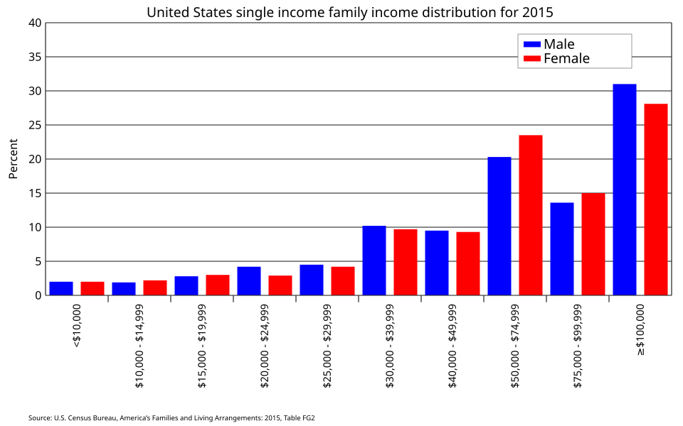bar chart of income distribution Monthly income distribution bar chart (Image: Delphi234, CC0, via Wikimedia Commons)

Based on the TU BBM syllabus for Business Statistics (STT201), unit 2.

Discussion

Loading…