Measures of Skewness & Kurtosis – concepts, formulas, interpretation, examples

1. What is Skewness?

Skewness quantifies the asymmetry of a frequency distribution around its central point.

• Positive skew (right‑skewed): long tail to the right, mean > median > mode.
• Negative skew (left‑skewed): long tail to the left, mean < median < mode.
• Zero skew: perfectly symmetric (e.g., normal distribution).

1.1 Pearson’s First Coefficient (Mode‑Based)

$$S_1=\frac{\mu -\text{Mode}}{\sigma }$$

1.2 Pearson’s Second Coefficient (Mean‑Median)

$$S_2=3\frac{\mu -\tilde{x}}{\sigma }$$

1.3 Bowley’s (Quartile) Coefficient

$$S_B=\frac{Q_3+Q_1-2\tilde{x}}{Q_3-Q_1}$$

where $Q_1$ and $Q_3$ are the first and third quartiles.

2. What is Kurtosis?

Kurtosis describes the tailedness and peak of a distribution relative to the normal curve.

$$K=\frac{{\mu }_4}{{\sigma }^4}=\frac{\sum (x_i-\mu {)}^4}{n{\sigma }^4}$$

• Leptokurtic ($K_e>0$): sharp peak, heavy tails (more outliers).
• Mesokurtic ($K_e=0$): same shape as normal distribution.
• Platykurtic ($K_e<0$): flat peak, light tails (fewer outliers).

2.1 Percentile (Bowley) Kurtosis

Using the 10th, 25th, 75th, and 90th percentiles:

$$K_p=\frac{(P_{90}-P_{10})}{(P_{75}-P_{25})}$$

A value > 2.7 suggests leptokurtic; < 2.7 suggests platykurtic.

3. Step‑by‑Step Computation (Flowchart)

flowchart TD
    A["Start: Collect raw data"] --> B["Compute mean (μ), median (M), mode (Mo)"]
    B --> C["Calculate standard deviation (σ)"]
    C --> D["Choose skewness formula"]
    D -->|"Pearson 1"| E["S1 = (μ‑Mo)/σ"]
    D -->|"Pearson 2"| F["S2 = 3(μ‑M)/σ"]
    D -->|"Bowley"| G["SB = (Q3+Q1‑2M)/(Q3‑Q1)"]
    E --> H["Interpret sign & magnitude"]
    F --> H
    G --> H
    H --> I["Compute fourth central moment"]
    I --> J["K = μ4 / σ⁴"]
    J --> K["Excess kurtosis Ke = K‑3"]
    K --> L["Interpret tail‑weight"]
    L --> M["End"]

4. Worked Example – Skewness (Pearson 2)

Problem (adapted from past exam):
Calculate Pearson’s second coefficient of skewness for a set of 100 families with the following income distribution.

4.1 Compute Mid‑points & Totals

$$\mu =\frac{\sum f_i{x}_i}{N}=\frac{5160}{100}=51.6$$

4.2 Median (M)

Cumulative frequencies: 13, 34, 61, 84, 100.
Median lies in the 40‑60 class (cumulative 34 → 61).

$$M=L+\left(\frac{\frac{N}{2}-C{F}_{prev}}{f}\right)h$$ where $L=40$, $C{F}_{prev}=34$, $f=27$, $h=20$.

$$M=40+\left(\frac{50-34}{27}\right)20=40+\frac{16}{27}\times 20\approx 51.85$$

4.3 Standard Deviation (σ)

$$\sigma =\sqrt{\frac{\sum f_i(x_i-\mu {)}^2}{N}}$$

Compute $(x_i-\mu {)}^2$ and multiply by $f_i$:

$$\sigma =\sqrt{\frac{67854}{100}}=\sqrt{678.54}\approx 26.05$$

4.4 Pearson’s Second Skewness

$$S_2=3\frac{\mu -M}{\sigma }=3\frac{51.6-51.85}{26.05}=3\frac{-0.25}{26.05}\approx -0.029$$

Interpretation: The coefficient is very close to zero (‑0.03), indicating an almost symmetric income distribution for these families.

5. Worked Example – Kurtosis (Percentile Method)

Problem (exam style):
From the marks distribution of a campus, calculate the percentile coefficient of kurtosis and interpret.

5.1 Determine Percentiles

Cumulative frequencies: 50, 150, 300, 390, 450, 500.

• 10th percentile (P10) lies in the 0‑10 class:
  $$P_{10}=L+\left(\frac{0.10N-C{F}_{prev}}{f}\right)h=0+\frac{50-0}{50}\times 10=10$$

• 90th percentile (P90) lies in the 40‑50 class (cumulative 450 → 500).
  $$P_{90}=40+\left(\frac{0.90N-450}{50}\right)10=40+\frac{450-450}{50}\times 10=40$$

• 25th percentile (Q1): 0.25 × 500 = 125 → falls in 10‑20 class.
  $$Q_1=10+\left(\frac{125-50}{100}\right)10=10+7.5=17.5$$

• 75th percentile (Q3): 0.75 × 500 = 375 → falls in 30‑40 class.
  $$Q_3=30+\left(\frac{375-300}{90}\right)10\approx 30+8.33=38.33$$

5.2 Percentile Kurtosis

$$K_p=\frac{P_{90}-P_{10}}{Q_3-Q_1}=\frac{40-10}{38.33-17.5}=\frac{30}{20.83}\approx 1.44$$

Interpretation:
The benchmark for a normal distribution is about 2.7. A value of 1.44 < 2.7 indicates a platykurtic distribution—flatter than normal, with relatively few extreme marks. This suggests the exam was moderate in difficulty, producing few very high or very low scores.

6. Comparison of Skewness & Kurtosis Measures

7. Advantages, Disadvantages & Applications

8. In the real world

• eSewa & Khalti transaction amounts: Daily payment totals show a right‑skewed pattern because a few large merchants generate high‑value transactions while most users make small payments. Pearson 2 skewness helps the platforms set tiered transaction fees.
• Daraz order queue: The time between order arrivals follows a leptokurtic distribution (high excess kurtosis). This indicates occasional bursts of orders during festivals, prompting Daraz to allocate extra delivery staff.
• NEPSE daily returns: Analysts compute excess kurtosis of stock‑return series. A high positive kurtosis signals heavy tails, warning investors about the probability of extreme price swings.

Worked tie‑in: The skewness example above (family income) mirrors the income‑distribution analysis performed by Nepal Bank Limited when designing loan products. A near‑zero skewness suggests a balanced client base, allowing the bank to set uniform interest rates rather than tiered ones.

9. Common Exam Pitfalls & How to Avoid Them

1. Mixing up formulas – always verify whether the question asks for Pearson 1, Pearson 2, or Bowley. Look for the presence of mode, median, or quartiles.
2. Incorrect percentile interpolation – use the class‑width method shown in the examples; do not assume the percentile equals the class lower bound.
3. Forgetting the “‑3” when the question asks for excess kurtosis.
4. Rounding too early – keep intermediate results to at least four decimal places; final answer is usually required to two decimals.
5. Skipping the interpretation – marks are awarded for stating whether the distribution is symmetric, positively/negatively skewed, leptokurtic, etc.

10. Exam tip

• Read the data table carefully; note whether frequencies are given as “below”, “and above”, or in class intervals.
• Identify the required coefficient from keywords: mode → Pearson 1, median → Pearson 2, quartiles → Bowley; percentiles → percentile kurtosis.
• Follow the flowchart: mean → median → mode → σ → apply formula → interpret. A one‑line checklist on your scrap paper saves time.
• Always write the interpretation (e.g., “S = 0.45 → moderately right‑skewed”). Examiners award marks for the comment.

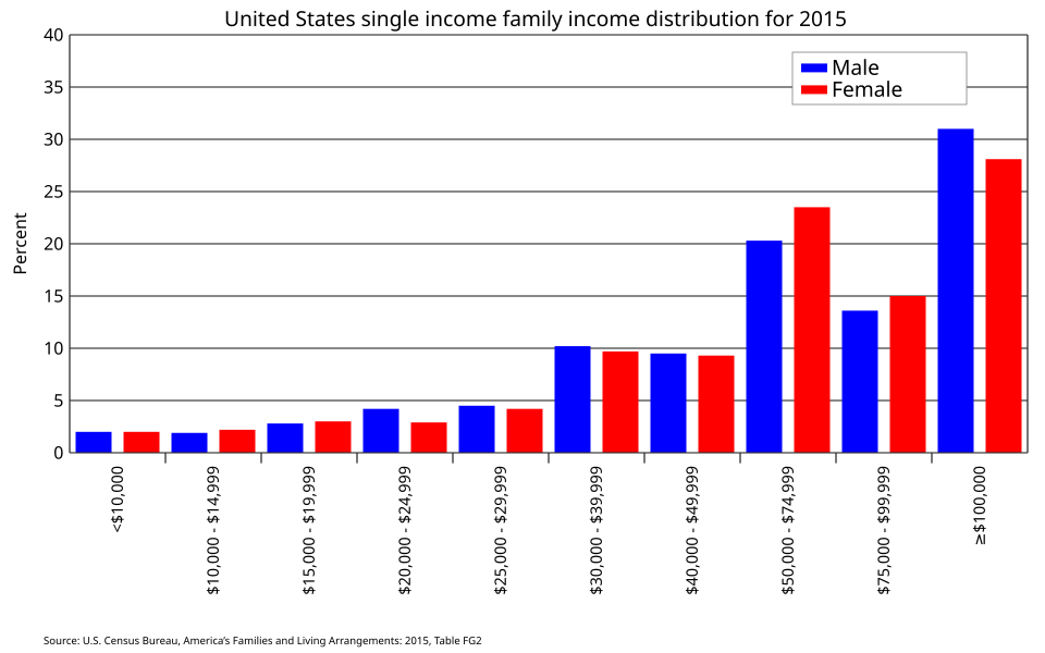Histogram illustrating the income classes and frequencies used in the skewness example (Image: Delphi234, CC0, via Wikimedia Commons)

End of Unit 6 notes – master these concepts and you’ll confidently tackle any skewness or kurtosis question in the TU Business Statistics exam.

In the real world

• eSewa Transaction Amounts: The platform uses Pearson’s Second Skewness to analyze transaction data. Most users make small payments (e.g., Rs. 100–500), but a few high-value transactions (e.g., Rs. 10,000+) skew the distribution rightward. This helps eSewa set dynamic transaction fees based on skewness thresholds.

• Nepal Rastra Bank (NRB) Risk Modeling: Banks apply excess kurtosis (Kₑ) to assess financial risk. A leptokurtic distribution (Kₑ > 0) in loan defaults signals higher-than-expected extreme losses, prompting stricter lending criteria. For example, if default data shows Kₑ = 1.8, NRB may adjust capital reserves accordingly.

• NEPSE Stock Market Analysis: Investors use Bowley’s Skewness to evaluate stock returns. A negative skew (e.g., S_B = -0.4) in a sector like hydropower suggests frequent small gains but occasional large drops, guiding portfolio diversification strategies.