Business StatisticsUnit 814 min read
Hypothesis Testing: Steps, Tests & Real-World Applications
Unit 8 of Business Statistics covers hypothesis testing—how to frame null/alternative hypotheses, choose significance levels, perform one/two-tailed tests, interpret p-values, and apply tests like z-test, t-test, and chi-square. Includes real-world examples from eSewa, Ncell, and Daraz.
TAKEAWAYS:
- Hypothesis testing follows a structured 5-step process: state hypotheses, choose significance level, select test statistic, compute test statistic, and make a decision.
- Type I (α) and Type II (β) errors are critical: α is rejecting a true null hypothesis (false positive), while β is failing to reject a false null (false negative).
- Test selection depends on data type: z-test for large samples (n ≥ 30) with known σ, t-test for small samples or unknown σ, and chi-square for categorical data.
- p-value interpretation: If p ≤ α, reject H₀; if p > α, fail to reject H₀. Common α levels: 0.05 (95% confidence) or 0.01 (99% confidence).
- Real-world applications: Banks use hypothesis testing to compare loan default rates (e.g., NMB vs. Global IME), eSewa tests if transaction success rates differ by region, and Daraz analyzes if promotional discounts significantly boost sales.
- Common mistakes: Misinterpreting H₀/H₁, ignoring assumptions (e.g., normality for t-tests), or using the wrong test (e.g., chi-square for continuous data).
1. Introduction to Hypothesis Testing
Hypothesis testing is a statistical method used to make decisions or inferences about a population based on sample data. It helps businesses, researchers, and policymakers answer questions like:
- "Does a new marketing campaign increase sales?" (eSewa’s referral bonuses)
- "Are two brands’ product lifespans significantly different?" (Ncell vs. NTC battery life)
- "Does a training program improve employee performance?" (Daraz delivery agents’ accuracy)
Key Definitions
- Null Hypothesis (H₀): Assumes no effect or no difference. Default assumption (e.g., "The mean salary of TU students is equal to Rs. 40,000").
- Alternative Hypothesis (H₁ or Ha): Claims there is an effect/difference. Can be:
- Two-tailed: "≠" (e.g., "The mean is not equal to Rs. 40,000").
- One-tailed (left/right): "<" or ">" (e.g., "The mean is less than Rs. 40,000").
- Significance Level (α): Probability of rejecting H₀ when it’s true (e.g., α = 0.05 means 5% risk of false rejection).
- Test Statistic: Standardized value (z, t, χ²) calculated from sample data to compare against critical values.
- p-value: Probability of observing the test statistic (or more extreme) if H₀ is true. Lower p-value → stronger evidence against H₀.
Visual: Hypothesis Testing Process Flow
flowchart TD
    A["Start"] --> B["State H₀ and H₁"]
    B --> C["Choose α (e.g., 0.05)"]
    C --> D["Select test (z, t, χ²)"]
    D --> E["Compute test statistic"]
    E --> F["Find critical value or p-value"]
    F --> G["Decision: Reject H₀ or Fail to Reject H₀"]
    G --> H["Conclusion"]
2. Steps of Hypothesis Testing
Step-by-Step with Example: eSewa Transaction Success Rates
Scenario: eSewa claims its transaction success rate is 98%. A sample of 200 transactions shows 188 successes. Test if the success rate is significantly different from 98% at α = 0.05.
Step 1: State Hypotheses
- H₀: p = 0.98 (success rate is 98%)
- H₁: p ≠ 0.98 (success rate is not 98%) → Two-tailed test
Step 2: Choose Significance Level
- α = 0.05 (5% risk of false rejection)
Step 3: Select Test Statistic
- Population proportion test (since data is categorical: success/failure).
- Use z-test (large sample: n × p = 200 × 0.98 = 196 ≥ 10, n × (1–p) = 4 ≥ 10).
Step 4: Compute Test Statistic
Formula for z-test for proportion: Where:
- = sample proportion = 188/200 = 0.94
- = hypothesized proportion = 0.98
- = sample size = 200
Calculation:
Step 5: Find Critical Value or p-value
- Critical value approach: For α = 0.05 (two-tailed), critical z-values are ±1.96. Since |–4.04| > 1.96, reject H₀.
- p-value approach: p-value = P(Z < –4.04 or Z > 4.04) ≈ 0.00005 (from z-table). Since p-value (0.00005) < α (0.05), reject H₀.
Step 6: Decision and Conclusion
- Decision: Reject H₀.
- Conclusion: There is sufficient evidence at α = 0.05 to say eSewa’s transaction success rate is not 98%.
3. Types of Hypothesis Tests
| Test | When to Use | Formula | Example |
|---|---|---|---|
| z-test | Large sample (n ≥ 30), known σ, or testing proportion. | Testing if Ncell’s average call duration (σ known) differs from 3 minutes. | |
| t-test | Small sample (n < 30), σ unknown, normally distributed data. | Comparing Daraz’s delivery times before/after hiring more agents. | |
| Chi-square (χ²) test | Categorical data (e.g., counts in categories). | Testing if Kathmandu traffic violations are equally distributed by district. | |
| ANOVA | Compare means of 3+ groups. | Comparing sales performance of 3 NMB bank branches. | |
| Regression t-test | Test if regression slope (β) is zero (no relationship). | Testing if eSewa’s promotional spend (X) affects transaction success (Y). |
4. Errors in Hypothesis Testing
| Error Type | Definition | Probability | Example |
|---|---|---|---|
| Type I (α) | Rejecting a true H₀ (false positive). | α (e.g., 5%) | Firing a loyal employee because a test falsely showed "low performance." |
| Type II (β) | Failing to reject a false H₀ (false negative). | Depends on power (1–β) | Approving a faulty batch of NTC bulbs because the test missed defects. |
| Power | Probability of correctly rejecting a false H₀ (1–β). Higher power = better test. | 1–β | A well-designed test for Daraz’s app crashes has 90% power to detect issues. |
Trade-off: Reducing α (e.g., to 0.01) lowers Type I error but increases Type II error.
5. Real-World Applications
Example 1: Ncell vs. NTC Battery Life (Two-Sample t-test)
Scenario: Ncell claims its phone batteries last longer than NTC’s. A sample of 15 Ncell and 12 NTC users gives:
- Ncell: hours,
- NTC: hours,
Test: Is Ncell’s battery life significantly longer at α = 0.05?
Steps:
- H₀: μ₁ ≤ μ₂ (Ncell ≤ NTC) H₁: μ₁ > μ₂ (Ncell > NTC) → One-tailed test.
- Test: Independent two-sample t-test (equal variances assumed).
- Formula: Where = pooled standard deviation.
- Calculation:
- Critical value: For df = 25, one-tailed α = 0.05 → .
- Decision: |1.12| < 1.708 → Fail to reject H₀.
- Conclusion: No significant evidence that Ncell’s battery lasts longer.
Example 2: Daraz’s Promotional Discounts (Regression t-test)
Scenario: Daraz wants to know if promotional discounts (X) significantly increase sales (Y). Data for 6 months:
| Discount (%) | Sales (Rs. '000) |
|---|---|
| 10 | 200 |
| 15 | 220 |
| 20 | 250 |
| 25 | 280 |
| 30 | 300 |
| 35 | 320 |
Test: Is the slope (β₁) of the regression line Y = β₀ + β₁X significantly different from 0?
Steps:
- Regression equation: Using Excel/calculator, find β₁ ≈ 5.71.
- H₀: β₁ = 0 (no relationship) H₁: β₁ ≠ 0 (relationship exists) → Two-tailed test.
- t-test for slope: From regression output: , so .
- Critical value: For df = 4 (n–2), α = 0.05 → .
- Decision: |7.14| > 2.776 → Reject H₀.
- Conclusion: Discounts significantly increase sales.
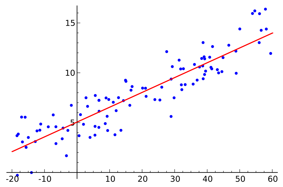 Daraz’s discount vs. sales data (Image: Sewaqu, Public domain, via Wikimedia Commons)
6. Chi-Square Test: Kathmandu Traffic Violations
Scenario: Police suspect traffic violations are not equally distributed across 4 districts (Lalitpur, Kageshwori, Chabahil, Thapathali). Observed violations:
| District | Observed (O) | Expected (E) = 100 |
|---|---|---|
| Lalitpur | 120 | 100 |
| Kageshwori | 80 | 100 |
| Chabahil | 90 | 100 |
| Thapathali | 110 | 100 |
Test: Are violations uniformly distributed? (α = 0.05)
Steps:
- H₀: Violations are uniformly distributed (E = 100 for each). H₁: Not uniformly distributed.
- Test: Chi-square goodness-of-fit test.
- Formula:
- Calculation:
- Critical value: For df = 3 (districts – 1), α = 0.05 → .
- Decision: 8 > 7.815 → Reject H₀.
- Conclusion: Violations are not uniformly distributed.
7. Exam Tip: How to Score Full Marks
- Show all steps: Examiners deduct marks for missing hypotheses, test selection, or calculations.
- Label clearly: Write "H₀:", "H₁:", "α =", "Test statistic:", etc.
- Use correct formulas: Memorize z, t, and χ² formulas. For regression, show both coefficients.
- Interpret results: Don’t just say "reject H₀"—explain what it means in context (e.g., "eSewa’s success rate is significantly different from 98%").
- Watch assumptions:
- z-test: Large sample or known σ.
- t-test: Normality (check with histogram/Q-Q plot if sample < 30).
- Chi-square: Expected frequencies ≥ 5 in each cell.
- Common pitfalls:
- Using one-tailed when two-tailed is needed (or vice versa).
- Ignoring degrees of freedom (df) for critical values.
- Misinterpreting p-values (e.g., "p = 0.06 means significant" is wrong).
8. Practice Questions (Exam-Style)
- NEPSE Stock Returns: A sample of 25 stocks has a mean return of 8% with s = 2%. Test if the population mean return is not 7% at α = 0.01.
- Bank Loan Defaults: Global IME claims its loan default rate is 5%. A sample of 200 loans has 14 defaults. Test at α = 0.05.
- Pathao vs. Uber: Pathao’s average ride time is 12 minutes (s = 2, n = 30). Uber’s is 11.5 minutes (s = 1.5, n = 35). Test if Pathao’s rides take longer at α = 0.05.
- Chi-square: A die is rolled 60 times with observed frequencies: 1→8, 2→12, 3→7, 4→10, 5→12, 6→11. Test fairness (α = 0.05).
9. Summary Table: Test Selection Guide
| Scenario | Test | Key Assumptions |
|---|---|---|
| Test proportion (e.g., success rate) | z-test for proportion | n × p ≥ 10, n × (1–p) ≥ 10 |
| Compare 2 means (large sample) | z-test | σ known or n ≥ 30 |
| Compare 2 means (small sample) | t-test (independent) | Normality, equal variances (if unknown) |
| Compare >2 means | ANOVA | Normality, equal variances |
| Categorical data (e.g., counts) | Chi-square | Expected frequencies ≥ 5 |
| Regression slope | t-test for β₁ | Linearity, normality of residuals |
In the real world
- eSewa: Uses z-tests for proportions to compare transaction success rates across regions (e.g., Kathmandu vs. Pokhara) to optimize referral bonuses. If the success rate in Pokhara (sample: 190/200) differs significantly from Kathmandu’s claimed 98%, they adjust promotions.
- NMB Bank: Applies t-tests to compare loan default rates between urban (σ unknown, n=50) and rural (n=30) branches. A t-statistic of 2.1 (p=0.04) at α=0.05 would reject H₀ (no difference) and trigger risk-mitigation policies.
- Daraz: Employs ANOVA to test if sales growth differs across 3+ promotional discount tiers (e.g., 10%, 20%, 30%). If F > F-critical (e.g., 4.5 > 3.1), they conclude discounts significantly impact sales and allocate budgets accordingly.
Based on the TU BBM syllabus for Business Statistics (STT201), unit 8.
Discussion
Loading…