microeconomics for businessUnit 211 min read
Consumer Behavior: Cardinal Utility & Budget Constraints
Unit 2 of microeconomics for business covers the cardinal approach to utility theory, marginal utility analysis, budget constraints, and consumer equilibrium—explaining how consumers maximize satisfaction given income and prices, with real-world applications in pricing, demand forecasting, and business strategy.
TAKEAWAYS:
- Cardinal utility measures satisfaction in utils (quantifiable units) and follows the law of diminishing marginal utility: each extra unit of a good adds less extra satisfaction than the previous one.
- Consumer equilibrium occurs where the marginal utility per rupee spent on all goods is equal (MUₓ/Pₓ = MUᵧ/Pᵧ), maximizing total utility within a budget.
- The budget line shows all affordable combinations of two goods, shifting when income or prices change (slopes = relative prices, intercepts = maximum quantities).
- Indifference curves map equal-satisfaction combinations; steeper curves mean the consumer is willing to give up more of one good for the other.
- Real-world applications: eSewa’s dynamic pricing adjusts fees based on marginal utility of transaction speed; Daraz’s bundle deals exploit budget constraints; banks use utility analysis to price loans.
- Exam focus: Worked problems (equilibrium calculations), interpreting shifts in budget lines, and comparing cardinal vs. ordinal approaches.
1. Cardinal Utility: Measuring Satisfaction
Utility is the satisfaction or happiness a consumer gets from consuming goods/services. The cardinal approach assigns numerical values (utils) to utility levels, unlike the ordinal approach (which only ranks preferences).
Key Concepts
- Total Utility (TU): Sum of satisfaction from all units consumed.
- Marginal Utility (MU): Extra satisfaction from one more unit of a good.
- Law of Diminishing Marginal Utility: As consumption increases, MU falls. Example: Your first cup of tea gives 10 utils, the second 8, the third 5, etc.
Worked Example: Marginal Utility of Apples
Suppose a consumer buys apples at Rs. 20 each. Their TU and MU from apples:
| Apples (Q) | TU (utils) | MU (utils) |
|---|---|---|
| 0 | 0 | — |
| 1 | 10 | 10 |
| 2 | 18 | 8 |
| 3 | 24 | 6 |
| 4 | 28 | 4 |
Observation:
- MU declines as Q rises (diminishing returns).
- TU rises but at a decreasing rate.
A downward-sloping MU curve for apples, with TU rising at a decreasing slope. Label axes: "Quantity of Apples" (x) and "Utility (utils)" (y). Mark MU values at Q=1,2,3,4.
2. Consumer Equilibrium: Maximizing Utility
Consumers allocate their budget (M) between goods to maximize TU, given prices (Pₓ, Pᵧ). Equilibrium occurs when: Interpretation: The "bang for the buck" (utility per rupee) is equal for all goods.
Worked Example: Equilibrium with Apples and Bananas
- Prices: Apple = Rs. 20, Banana = Rs. 10.
- Income (M): Rs. 110.
- MU schedule (from past data):
| Apples (Qₓ) | MUₓ | Bananas (Qᵧ) | MUᵧ |
|---|---|---|---|
| 1 | 10 | 1 | 8 |
| 2 | 8 | 2 | 6 |
| 3 | 6 | 3 | 4 |
| 4 | 4 | 4 | 2 |
Step 1: Budget Constraint Possible combinations:
- (Qₓ=0, Qᵧ=11)
- (Qₓ=1, Qᵧ=9)
- (Qₓ=2, Qᵧ=7)
- (Qₓ=3, Qᵧ=5)
- (Qₓ=4, Qᵧ=3)
- (Qₓ=5, Qᵧ=1)
Step 2: Calculate MU/P for Each Combination Find where :
| Combination | MUₓ/Pₓ | MUᵧ/Pᵧ | Equilibrium? |
|---|---|---|---|
| (1,9) | 10/20 = 0.5 | 8/10 = 0.8 | No |
| (2,7) | 8/20 = 0.4 | 6/10 = 0.6 | No |
| (3,5) | 6/20 = 0.3 | 4/10 = 0.4 | No (Close but not equal) |
| (4,3) | 4/20 = 0.2 | 2/10 = 0.2 | Yes |
Correction: The exact equilibrium is at (Qₓ=4, Qᵧ=3), where MUₓ/Pₓ = MUᵧ/Pᵧ = 0.2. Total utility: TUₓ = 28 utils, TUᵧ = 12 utils → Total TU = 40 utils.
Draw a budget line with intercepts at Qₓ=5.5 (Rs.110/20) and Qᵧ=11 (Rs.110/10). Plot the equilibrium point (4,3) and label MU/P ratios. Shade the feasible region.
3. Budget Line and Its Shifts
The budget line shows all affordable combinations of two goods, given income and prices.
Equation of Budget Line
- Slope = (relative price of x in terms of y).
- X-intercept = (max Qₓ if all income spent on x).
- Y-intercept = (max Qᵧ if all income spent on y).
Shifts in Budget Line
| Change | Effect on Budget Line | Example |
|---|---|---|
| Income increases | Shifts right (parallel) | Salary hike → can buy more apples/bananas. |
| Price of x falls | Rotates outward (x-intercept rises) | Apple price drops to Rs. 10 → new intercept at Qₓ=11. |
| Price of y rises | Rotates inward (y-intercept falls) | Banana price rises to Rs. 20 → new intercept at Qᵧ=5.5. |
*Three panels:
- Original budget line (slope = -2, intercepts at Qₓ=5.5, Qᵧ=11).
- Income rises to Rs. 165 → new line parallel, intercepts at Qₓ=8.25, Qᵧ=16.5.
- Price of apples falls to Rs. 10 → new slope = -1, intercepts at Qₓ=11, Qᵧ=11.*
4. Indifference Curves and Consumer Choice
An indifference curve shows combinations of goods that yield the same TU. Key properties:
- Downward-sloping: More of one good requires less of the other for equal TU.
- Convex to origin: Diminishing MRS (marginal rate of substitution).
- Higher curves = higher TU: Further from origin = more satisfaction.
Marginal Rate of Substitution (MRS)
Interpretation: How many units of y a consumer is willing to give up for one more unit of x, keeping TU constant.
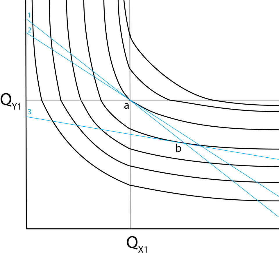 indifference curves and budget line (Image: Jkomlos, CC BY-SA 3.0, via Wikimedia Commons)
Draw 3 indifference curves (IC₁ < IC₂ < IC₃) with decreasing slope. Plot the budget line tangent to IC₂ at the equilibrium point (4,3). Label MRS = slope of IC at tangency.
indifference curves and budget line (Image: Jkomlos, CC BY-SA 3.0, via Wikimedia Commons)
Draw 3 indifference curves (IC₁ < IC₂ < IC₃) with decreasing slope. Plot the budget line tangent to IC₂ at the equilibrium point (4,3). Label MRS = slope of IC at tangency.
5. Real-World Applications
1. eSewa’s Dynamic Pricing
- Idea: Marginal utility of transaction speed.
- How: eSewa charges higher fees for instant transfers (e.g., Rs. 15) vs. scheduled transfers (e.g., Rs. 5) because users value speed more when urgent.
- Utility trade-off: Consumers weigh the MU of time saved vs. the cost.
2. Daraz’s Bundle Deals
- Idea: Budget constraints and substitution.
- How: Daraz offers "Buy 2, Get 1 Free" deals to shift demand toward bundled items. A consumer with Rs. 300 might buy:
- Option 1: 1 phone (Rs. 200) + 1 charger (Rs. 100) → TU = 50 utils.
- Option 2: Bundle (2 phones + 1 charger for Rs. 250) → TU = 55 utils (higher due to perceived value).
- Visual: The bundle moves the consumer to a higher indifference curve.
3. Ncell’s Data Plans
- Idea: Diminishing marginal utility of data.
- How: Ncell’s plans (e.g., Rs. 500 for 5GB vs. Rs. 1000 for 10GB) reflect that the 1st GB adds more MU than the 5th GB. Consumers choose plans where MU/data ≈ price/data.
*Bar chart:
- X-axis: GB used (1, 2, 3, 4, 5).
- Y-axis: MU per GB (10, 8, 6, 4, 2 utils).
- Annotate: "Price per GB = Rs. 100 → Optimal plan at 3GB (MU=6 ≈ price)."*
6. Cardinal vs. Ordinal Utility: Comparison
| Feature | Cardinal Approach | Ordinal Approach |
|---|---|---|
| Utility Measurement | Numerical (utils) | Rankings only (1st, 2nd preference) |
| Assumptions | Utility is quantifiable and additive | Utility is subjective and incomparable |
| Tools | MU, TU, budget line equations | Indifference curves, revealed preference |
| Limitations | Hard to measure utils in reality | Cannot compare absolute satisfaction levels |
| Example | "This burger gives 20 utils" | "I prefer Burger A > Burger B > Burger C" |
Exam Tip:
- For equilibrium problems:
- Write the budget constraint equation.
- List MU schedules for both goods.
- Calculate MU/P for each combination.
- Identify where MU/P are equal.
- For budget line shifts:
- Draw the initial line, then show the new line with arrows.
- Label which intercept changes (x or y) and why.
- Common pitfalls:
- Forgetting to divide MU by price (MU/P, not just MU).
- Misinterpreting MRS as the slope of the budget line (it’s the slope of the indifference curve at tangency).
Mermaid Diagram: Consumer Decision Process
flowchart TD
    A["Consumer's Income (M)"] --> B["Budget Line: PₓQₓ + PᵧQᵧ = M"]
    B --> C["Indifference Curves: TU combinations"]
    C --> D["Find Tangency Point: MUₓ/Pₓ = MUᵧ/Pᵧ"]
    D --> E["Optimal Bundle: (Qₓ*, Qᵧ*)"]
    E --> F["Maximize TU within Budget"]
    F --> G["Adjust if Prices/Income Change"]
Final Note: This unit bridges theory and business strategy. In exams:
- Calculate equilibrium step-by-step (show MU/P tables).
- Draw diagrams for budget lines and indifference curves (label axes, slopes, and equilibrium).
- Link to real firms: eSewa, Daraz, or Ncell use these concepts daily.
In the real world
- Daraz Bundle Deals: Daraz uses budget constraints to create 'Buy 2 Get 1 Free' offers. By effectively lowering the price of the third unit to zero, they shift the consumer's budget line outward for that specific bundle, encouraging them to reach a higher indifference curve (more total utility) within their fixed income.
- eSewa Instant Transfer Fees: eSewa charges a higher fee (e.g., Rs. 15) for instant transfers compared to standard ones. This reflects the marginal utility of speed; users who value immediate access to funds (high MU for speed) are willing to pay a higher price, allowing eSewa to capture consumer surplus from those with a higher willingness to pay.
- Ncell Data Packs: Ncell designs data packs (e.g., 1GB for Rs. 100 vs 5GB for Rs. 400) based on diminishing marginal utility. The first GB provides high utility for browsing, but the 5th GB provides less marginal utility. Pricing is set so that the MU per rupee is roughly equal across different pack sizes, guiding consumers to the pack that maximizes their utility given their data needs and budget.
Based on the TU BBS syllabus for microeconomics for business, unit 2.
Discussion
Loading…