microeconomics for businessUnit 89 min read
Economies of Scale, Scope, and Diseconomies: Cost Efficiency and Business Growth
Unit 8 of microeconomics for business explores how firms reduce per-unit costs by expanding production (economies of scale), diversifying products (economies of scope), and the challenges of overgrowth (diseconomies). It links these concepts to real-world business strategies, cost curves, and market performance.
TAKEAWAYS:
- Economies of scale reduce long-run average costs as output grows, driven by technical, managerial, or financial efficiencies.
- Economies of scope arise when producing multiple products together is cheaper than separately, measured by cost savings or scope economies index.
- Diseconomies of scale occur when expansion leads to inefficiencies like coordination failures or bureaucratic costs.
- Minimum efficient scale (MES) is the output level where all scale economies are exhausted, critical for market entry decisions.
- Real-world examples: Daraz’s warehouse consolidation (scale), Google’s Android + Chrome (scope), and Ncell’s network congestion (diseconomies).
- Exam focus: Define, calculate, and compare scale/scope/diseconomies using cost curves, numerical examples, and business cases.
1. Economies of Scale: Why Bigger Firms Can Produce Cheaper
Economies of scale occur when a firm’s long-run average total cost (LRATC) falls as output increases. This happens because larger production allows firms to exploit efficiencies that smaller firms cannot. There are three main types:
Types of Economies of Scale
mindmap
  root((Economies of Scale))
    Technical
      Specialization of labor
      Bulk purchasing of inputs
      Advanced machinery
    Managerial
      Better coordination
      Division of labor
    Financial
      Lower interest rates (larger loans)
      Tax benefits
    Marketing
      Brand recognition (e.g., Daraz’s nationwide ads)
    Risk-bearing
      Spreading fixed costs (e.g., NTC’s network infrastructure)
How It Works: Cost Curves and Scale
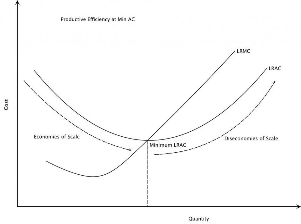
The long-run average cost (LRAC) curve slopes downward initially due to economies of scale, then flattens at the minimum efficient scale (MES), and may rise if diseconomies set in.
Worked Example: Daraz’s Warehouse Expansion
- Scenario: Daraz opens a new warehouse in Kathmandu to serve 50,000 daily orders.
- Costs at Small Scale (10,000 orders/day):
- Rent: Rs. 500,000/month
- Staff: 20 workers @ Rs. 20,000 each = Rs. 400,000/month
- ATC = (Rs. 900,000)/(10,000 orders) = Rs. 90/order
- Costs at Large Scale (50,000 orders/day):
- Rent: Rs. 1,000,000/month (bulk discount)
- Staff: 50 workers @ Rs. 18,000 each = Rs. 900,000/month (specialized roles)
- Machinery: Rs. 2,000,000 one-time (amortized over 5 years)
- ATC = (Rs. 3,900,000 + Rs. 400,000)/(50,000 orders) ≈ Rs. 82/order
- Economy of Scale: ATC drops from Rs. 90 to Rs. 82, a 8.9% cost reduction per order.
Key Insight: Daraz’s expansion exploits technical economies (larger machinery) and managerial economies (specialized staff), but only up to a point—beyond 100,000 orders, coordination costs may rise.
2. Economies of Scope: Producing More Than One Product
Economies of scope occur when a firm can produce multiple products more cheaply together than separately. This is common in firms with shared resources (e.g., factories, brands, or distribution networks).
Measurement: Cost Savings and Scope Economies Index
The scope economies index (SEI) measures cost savings from joint production:
- SEI < 1: Economies of scope exist (joint production is cheaper).
- SEI = 1: No scope economies.
- SEI > 1: Diseconomies of scope (costly to produce together).
Worked Example: Google’s Android + Chrome
- Separate Costs:
- Developing Android OS: $500 million/year
- Developing Chrome browser: $300 million/year
- Total = $800 million
- Joint Costs:
- Shared R&D, marketing, and user data insights reduce costs to $600 million.
- SEI = 600 / 800 = 0.75 → 25% cost savings due to economies of scope.
Why It Matters for Nepalese Firms:
- Nepal Telecom (NTC): Offers internet + mobile bundles (shared network infrastructure).
- Banks: Cross-selling loans + insurance (shared customer data).
3. Diseconomies of Scale: When Bigger Becomes Costlier
Diseconomies of scale occur when a firm grows too large, leading to inefficiencies. These are internal (firm-specific) or external (market-wide).
Causes of Diseconomies
| Internal Diseconomies | External Diseconomies |
|---|---|
| Poor communication (e.g., Ncell’s HQ) | Rising input costs (e.g., NTC’s spectrum fees) |
| Bureaucracy (e.g., Daraz’s slow approvals) | Overcrowded markets (e.g., Kathmandu traffic) |
| Worker alienation (e.g., factory lines) | Government regulations (e.g., labor laws) |
| Coordination failures (e.g., NEPSE’s delayed trades) | Inflation reducing purchasing power |
Worked Example: Ncell’s Network Congestion
- Problem: Ncell’s rapid growth led to overloaded cell towers in busy areas (e.g., Thapathali).
- Costs:
- Before: Rs. 500 million/year for maintenance.
- After: Rs. 800 million/year due to extra towers and repairs.
- Diseconomy: ATC rises because external diseconomies (limited spectrum) force costly workarounds.
Visualizing Diseconomies:
4. Minimum Efficient Scale (MES): The Sweet Spot
The minimum efficient scale (MES) is the output level where a firm achieves all possible economies of scale and begins facing diseconomies. It determines:
- Market entry barriers: Firms below MES may struggle to compete.
- Optimal firm size: E.g., a Daraz warehouse’s MES might be 30,000 daily orders.
Example: Kathmandu Traffic Routes
- Small Scale: A single bus route (e.g., New Baneshwor to Thamel) has high ATC due to fixed costs (driver, fuel).
- MES: 50 buses/route (spreads costs, but adding more causes congestion).
- Diseconomies: Beyond 70 buses, delays increase ATC due to traffic jams.
5. Real-World Applications in Nepal and Globally
In the Real World
eSewa (Digital Payments)
- Economy of Scale: Processes millions of transactions/day at lower per-transaction costs due to bulk IT infrastructure.
- Diseconomy Risk: If eSewa grows too fast, fraud detection costs may rise (bureaucracy).
Pathao (Ride-Hailing)
- Economy of Scope: Uses the same app for rides + food delivery, reducing development costs.
- SEI Calculation: Joint app costs < separate apps for rides + delivery.
Nepal Rastra Bank (NRB)
- Economy of Scale: Single regulatory body for all banks reduces compliance costs for smaller banks.
- Diseconomy: If NRB becomes too centralized, slow decision-making may hurt financial markets.
Daraz vs. Local Shops
- Daraz’s Advantage: Economies of scale in warehousing, logistics, and bulk discounts from suppliers.
- Local Shops’ Disadvantage: Cannot achieve MES, so higher prices.
6. Comparing Scale, Scope, and Diseconomies
| Feature | Economies of Scale | Economies of Scope | Diseconomies of Scale |
|---|---|---|---|
| Definition | Lower ATC with larger output | Lower costs from producing multiple goods | Higher ATC due to overgrowth |
| Cause | Specialization, bulk purchasing | Shared resources (R&D, marketing) | Coordination failures, bureaucracy |
| Example (Nepal) | NTC’s nationwide fiber network | Ncell’s mobile + internet bundles | NEPSE’s delayed trading system |
| Measurement | % change in ATC with output growth | Scope Economies Index (SEI) | % increase in ATC after MES |
| Business Strategy | Expand production (e.g., Daraz) | Diversify products (e.g., Google) | Restructure or downsize (e.g., Ncell) |
Exam Tip
Define Clearly:
- Economies of scale = LRATC falls as output rises.
- Economies of scope = Joint production costs < separate costs.
- Diseconomies = LRATC rises due to inefficiencies.
Calculate Numerically:
- For scale: Show ATC before/after expansion (e.g., Daraz’s warehouse).
- For scope: Compute SEI using joint vs. separate costs (e.g., Google’s Android + Chrome).
Link to Real Firms:
- Scale: NTC, Daraz, banks.
- Scope: eSewa, Pathao, Ncell bundles.
- Diseconomies: NEPSE delays, Kathmandu traffic, Ncell congestion.
Draw Cost Curves:
- Always label:
- LRAC (U-shaped).
- MES (minimum point).
- Scale economies (falling part).
- Diseconomies (rising part).
- Always label:
Common Pitfalls:
- ❌ Confusing short-run (fixed plant) with long-run (variable plant) costs.
- ❌ Ignoring external diseconomies (e.g., inflation, regulations).
- ❌ Forgetting MES is where scale economies end.
Final Visual Summary:
Based on the TU BBS syllabus for microeconomics for business, unit 8.
Discussion
Loading…