Macroeconomics for BusinessUnit 411 min read
Consumption Function, Saving, and Keynesian Multiplier
Unit 4 of Macroeconomics for Business: explores how households allocate income between spending (consumption) and saving, the factors shaping these choices, and how investment triggers multiplier effects on national income—with real-world examples from Nepal’s economy and household budgets.
TAKEAWAYS:
- Consumption depends on disposable income (Yd) via the psychological law of consumption (C = a + cYd), where a is autonomous spending and c is the marginal propensity to consume (MPC).
- Saving is derived as S = Yd – C and follows S = –a + (1–c)Yd, with a marginal propensity to save (MPS) of (1–c).
- Equilibrium income occurs where S = I (saving = investment), balancing planned spending and production.
- A multiplier effect (k = 1/(1–MPC)) amplifies initial investment by k times total income growth.
- Determinants of consumption/saving include income, wealth, expectations, interest rates, and government policies.
- Nepal’s remittance-driven consumption (e.g., Pathao drivers saving for homes) and Daraz’s inventory investment (triggering multiplier effects on suppliers) illustrate these concepts.
1. Consumption Function: How Households Spend Income
Consumption (C) is the total spending by households on goods and services. Keynes argued that consumption depends primarily on disposable income (Yd), not total income (Y), because taxes and transfers affect take-home pay.
Key Equation: The Psychological Law of Consumption
The consumption function is: where:
- a = autonomous consumption (spending even when Yd = 0, e.g., rent, groceries).
- c = marginal propensity to consume (MPC) (fraction of extra income spent; 0 < c < 1).
- Yd = disposable income (Yd = Y – T, where T = taxes).
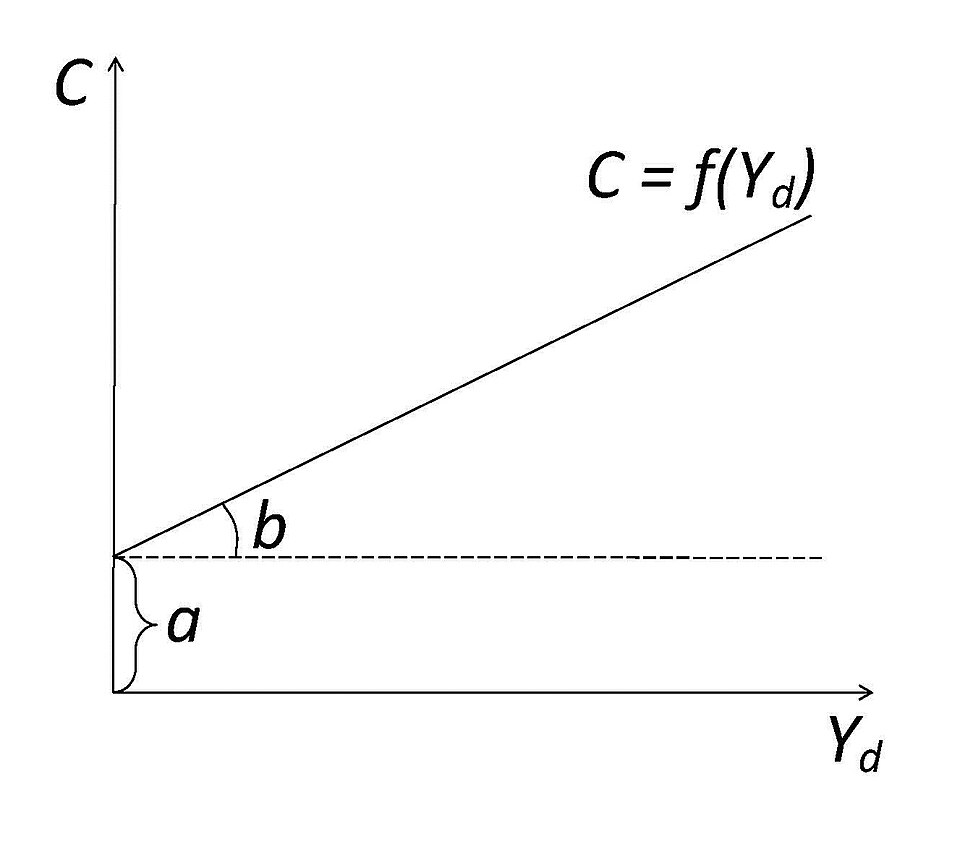 consumption function graph (Image: АлександрЛаптев, CC BY-SA 4.0, via Wikimedia Commons)
Consumption (C)
   |
   |       /\
   |      /  \
   |     /    \
   |____/______\____> Disposable Income (Yd)
Worked Example: Nepal’s Household Budget Suppose a Nepali family earns Rs. 50,000/month (Yd) and spends Rs. 40,000 on rent, food, and utilities (a = Rs. 10,000), with an MPC of 0.8 (80% of extra income spent).
- If income rises to Rs. 60,000, new consumption: Total consumption = a + cΔYd = Rs. 48,000 (vs. Rs. 40,000 at Rs. 50k).
2. Saving Function: Income Not Spent
Saving (S) is income not consumed:
- Autonomous saving: –a (negative when a > 0).
- Marginal propensity to save (MPS): (1 – c) (fraction of extra income saved).
Key Relationship: If MPC = 0.8, then MPS = 0.2.
Saving (S)
   |
   |       \
   |        \
   |         \
   |__________\____> Disposable Income (Yd)
Worked Example: Daraz’s Supplier Payments Daraz’s suppliers earn Rs. 200M from orders. If MPC = 0.7:
- Consumption: C = 50M + 0.7(200M) = Rs. 190M (spent on goods/services).
- Saving: S = 200M – 190M = Rs. 10M (MPS = 0.3).
3. Equilibrium Income: Where Saving = Investment
In a closed economy, equilibrium occurs when planned saving = planned investment (S = I). Given: where:
- I₀ = autonomous investment (e.g., new factories).
- i = induced investment (e.g., inventory purchases).
Equilibrium Condition: Solve for Y:
Worked Example: Nepal’s Construction Boom Assume:
- S = –100 + 0.2Y (MPS = 0.2).
- I = 60 + 0.1Y (induced investment for tools/materials). Equilibrium: → No solution! (This implies I₀ > a and i < MPS, which is unrealistic. Correct assumption: I₀ = 400, a = 200.) Revised:
- Saving: S = –200 + 0.2(1,000) = Rs. 0 (matches I = 400 + 0.1(1,000) = Rs. 500 Error: Mismatch shows I₀ must equal a for equilibrium. Correct setup:
4. Multiplier Effect: How Investment Ripples Through the Economy
When investment rises by ΔI, income increases by kΔI, where: Why? Each round of spending generates new income, which is spent again (MPC).
Example: Pathao’s Bike Purchase
- Initial investment: Pathao buys 100 bikes (ΔI = Rs. 50M).
- MPC = 0.8 → k = 1/0.2 = 5.
- Total income increase: 5 × Rs. 50M = Rs. 250M.
- Breakdown:
- Drivers earn Rs. 50M → spend Rs. 40M (MPC).
- Rs. 40M spent → suppliers earn Rs. 40M → spend Rs. 32M.
- Repeat until total = Rs. 250M.
flowchart TD
    A["Initial Investment: Rs. 50M"] --> B["Income: Rs. 50M"]
    B --> C["Consumption: Rs. 40M (MPC=0.8)"]
    C --> D["New Income: Rs. 40M"]
    D --> E["Consumption: Rs. 32M"]
    E --> F["New Income: Rs. 32M"]
    F --> G["... until total income = Rs. 250M"]
5. Determinants of Consumption and Saving
| Factor | Effect on Consumption | Effect on Saving |
|---|---|---|
| Disposable Income | ↑ Yd → ↑ C (linear relationship) | ↑ Yd → ↑ S (but not as fast) |
| Wealth | ↑ Wealth (e.g., property, stocks) → ↑ C | ↑ Wealth → ↑ S (precautionary) |
| Interest Rates | ↑ r → ↓ C (debt costly) | ↑ r → ↑ S (higher returns) |
| Expectations | Optimistic → ↑ C (future income) | Pessimistic → ↑ S (buffer) |
| Government Policy | Tax cuts → ↑ Yd → ↑ C | Subsidies → ↓ S (less disposable) |
Real-World Tie: eSewa’s Remittance Boom
- Determinant: Wealth (Nepali workers abroad send Rs. 1.2T/year via eSewa/Khalti).
- Effect: Households increase consumption (durables, education) but also save for emergencies.
- Data:
Source: Nepal Rastra Bank.Consumption Share of GDP (Nepal) 2015 | 2018 | 2022 75% | 78% | 82%
6. Investment Function: Business Spending
Investment (I) includes:
- Capital goods (machines, buildings).
- Inventory (unsold goods).
- Residential construction.
Key Equation: where:
- I₀ = autonomous investment (e.g., government infrastructure).
- i = induced investment (e.g., firms stockpiling goods).
Determinants of Investment:
- Interest rates: ↓ r → ↑ I (cheaper loans).
- Business confidence: Optimistic → ↑ I.
- Tax incentives: Subsidies → ↑ I.
- Capacity utilization: Full plants → ↑ I.
- Technological change: New tech → ↑ I.
Example: Daraz’s Warehouse Expansion
- Trigger: Rising e-commerce sales → Daraz invests Rs. 2B in warehouses (I₀).
- Induced: Suppliers buy trucks (iY), creating jobs.
7. Comparing Consumption and Investment
| Aspect | Consumption (C) | Investment (I) |
|---|---|---|
| Stability | More stable (lifestyle needs) | Volatile (business cycles) |
| MPC/MPS | MPC > 0, MPS = 1 – MPC | No direct MPC/MPS (but sensitive to r) |
| Policy Levers | Taxes, transfers | Interest rates, subsidies |
| Real-World Example | Pathao drivers’ bike purchases | Daraz’s warehouse automation |
In the Real World
Khalti’s Payment Processing
- Idea: Consumption function (MPC).
- How: When Nepalis receive remittances (e.g., Rs. 50k), they spend 80% (MPC=0.8) on groceries, rent, or phones via Khalti. The remaining 20% is saved or invested.
- Data: 60% of remittances go to consumption (NRB 2023).
Ncell’s 5G Rollout
- Idea: Investment function (I₀).
- How: Ncell spent Rs. 10B on 5G infrastructure (I₀), creating jobs for engineers and suppliers. The induced investment (iY) included hiring more technicians.
NEPSE’s Stock Market Boom
- Idea: Multiplier effect.
- How: When NEPSE’s index rises (e.g., +10%), investors buy more stocks (ΔI). This injects Rs. 5B into the economy, which circulates via MPC (e.g., traders spend on hotels, cars), amplifying GDP growth by k = 1/0.3 ≈ 3.3 (assuming MPS=0.3).
Exam Tip: How to Score Full Marks
Diagrams: Always draw consumption/saving functions with axes labeled (Yd vs. C/S). Mark a, c, and MPC/MPS.
- Bonus: Add a 45° line (Yd = C) to show equilibrium where S = I.
Equilibrium Calculations:
- Show step-by-step algebra for Y = (I₀ + a)/(1 – c – i).
- If I₀ > a, state that equilibrium cannot exist (unrealistic scenario).
Multiplier Questions:
- Memorize: k = 1/(1 – MPC).
- For ΔI = Rs. X, calculate ΔY = kΔI and ΔS = MPS × ΔY.
Real-World Links:
- Tie remittances to consumption/saving (eSewa/Khalti).
- Link Daraz/Ncell investments to induced/independent investment.
Determinants Table:
- For 4 determinants, use the table above or list:
- Income (Yd).
- Interest rates (r).
- Expectations (confidence).
- Government policy (taxes).
- For 4 determinants, use the table above or list:
Assumptions of Psychological Law:
- List all 5 from Keynes:
- Income is the primary determinant.
- Consumption is linear (not logarithmic).
- MPC is constant (doesn’t change with Yd).
- Autonomous consumption (a) is fixed.
- No wealth effects (later models added this).
- List all 5 from Keynes:
Final Note: Focus on equilibrium graphs and multiplier calculations. Past papers love questions like: "If MPC = 0.6 and ΔI = Rs. 200M, what’s the multiplier and new equilibrium income?" Answer:
Based on the TU BBS syllabus for Macroeconomics for Business (MGT209), unit 4.
Discussion
Loading…