Theorems of Calculus – MVT & Rolle's Theorem

Delivery driver transporting goods (Image: Meanwell Packaging, CC BY 2.0, via Wikimedia Commons)

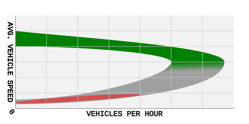Visual representation of traffic flow on a road (Image: HueSurname, CC BY-SA 4.0, via Wikimedia Commons)

Definitions

Rolle’s Theorem
Let $f:[a,b]\to \mathbb{R}$ satisfy

1. $f$ is continuous on $[a,b]$;
2. $f$ is differentiable on $(a,b)$;
3. $f(a)=f(b)$.
   Then there exists at least one $c\in (a,b)$ such that
   $$f^{\prime }(c)=0.$$

Mean Value Theorem (Lagrange’s MVT)
Let $f:[a,b]\to \mathbb{R}$ satisfy

1. $f$ is continuous on $[a,b]$;
2. $f$ is differentiable on $(a,b)$.
   Then there exists at least one $c\in (a,b)$ such that
   $$f^{\prime }(c)=\frac{f(b)-f(a)}{b-a}.$$

The right‑hand side is the average rate of change of $f$ on $[a,b]$.

Geometrical Interpretation

• Rolle’s Theorem: If a curve starts and ends at the same height over an interval, the tangent line must be horizontal somewhere in between.
• MVT: The slope of the secant line joining $(a,f(a))$ and $(b,f(b))$ equals the slope of the tangent at some interior point.

These interpretations are illustrated in the following figures.

Proof Sketches

Rolle’s Theorem

1. Define $g(x)=f(x)-f(a)$.
2. Then $g(a)=g(b)=0$.
3. By the Extreme Value Theorem, $g$ attains a maximum or minimum on $[a,b]$.
4. At an interior extremum, $g^{\prime }(c)=0$.
5. Hence $f^{\prime }(c)=0$.

Mean Value Theorem

1. Construct
   $$g(x)=f(x)-\frac{f(b)-f(a)}{b-a}(x-a).$$
2. Observe $g(a)=g(b)=0$.
3. Apply Rolle’s Theorem to $g$ on $[a,b]$.
4. There exists $c\in (a,b)$ with $g^{\prime }(c)=0$.
5. Compute
   $$g^{\prime }(x)=f^{\prime }(x)-\frac{f(b)-f(a)}{b-a}=0⟹f^{\prime }(c)=\frac{f(b)-f(a)}{b-a}.$$

The flow of the MVT proof is summarised below.

flowchart TD
  "Define g(x)" --> "Check g(a)=g(b)=0"
  "Check g is continuous on [a,b] and differentiable on (a,b)" --> "Apply Rolle's Theorem"
  "=> There exists c in (a,b) with g'(c)=0" --> "=> f'(c) = (f(b)-f(a))/(b-a)"

Worked Examples

1. Verify MVT for $f(x)=x^3+x^2-6x$ on $[-1,4]$.

1. Check conditions: $f$ is a polynomial → continuous and differentiable everywhere.
2. Compute average rate:
   $$\frac{f(4)-f(-1)}{4-(-1)}=\frac{(64+16-24)-(-1+1+6)}{5}=\frac{56-6}{5}=10.$$
3. Find $f^{\prime }(x)$:
   $$f^{\prime }(x)=3x^2+2x-6.$$
4. Solve $f^{\prime }(c)=10$:
   $$3c^2+2c-6=10\Rightarrow 3c^2+2c-16=0.$$
   Using quadratic formula:
   $$c=\frac{-2\pm \sqrt{4+192}}{6}=\frac{-2\pm \sqrt{196}}{6}=\frac{-2\pm 14}{6}.$$
   Two solutions: $c=2$ and $c=-\frac{8}{3}$.
5. Check interval: Only $c=2$ lies in $(-1,4)$.
6. Conclusion: MVT holds with $c=2$.

Graphical confirmation: The secant line between $(-1,f(-1))$ and $(4,f(4))$ has slope $10$; the tangent at $x=2$ also has slope $10$.

2. Verify Rolle’s Theorem for $f(x)=\sin x$ on $[0,\pi ]$.

1. Conditions: $\sin x$ is continuous and differentiable everywhere.
2. Endpoint values: $f(0)=0=f(\pi )$.
3. Derivative: $f^{\prime }(x)=\cos x$.
4. Solve $f^{\prime }(c)=0$: $\cos c=0$ ⇒ $c=\frac{\pi }{2}$.
5. Check interval: $\frac{\pi }{2}\in (0,\pi )$.
6. Conclusion: Rolle’s Theorem holds with $c=\frac{\pi }{2}$.

3. Verify Rolle’s Theorem for $f(x)=x^2-9$ on $[-3,3]$.

1. Endpoint values: $f(-3)=0=f(3)$.
2. Derivative: $f^{\prime }(x)=2x$.
3. Solve $f^{\prime }(c)=0$: $c=0$.
4. Conclusion: Rolle’s Theorem holds with $c=0$.

4. Verify Lagrange’s MVT for $f(x)=\sqrt{x-1}$ on $[1,3]$.

1. Conditions: $f$ is continuous on $[1,3]$ and differentiable on $(1,3)$.
2. Average rate:
   $$\frac{f(3)-f(1)}{3-1}=\frac{\sqrt{2}-0}{2}=\frac{\sqrt{2}}{2}.$$
3. Derivative:
   $$f^{\prime }(x)=\frac{1}{2\sqrt{x-1}}.$$
4. Solve $f^{\prime }(c)=\frac{\sqrt{2}}{2}$:
   $$\frac{1}{2\sqrt{c-1}}=\frac{\sqrt{2}}{2}\Rightarrow \sqrt{c-1}=\frac{1}{\sqrt{2}}\Rightarrow c-1=\frac{1}{2}\Rightarrow c=\frac{3}{2}.$$
5. Conclusion: MVT holds with $c=\frac{3}{2}$.

Comparison Table

Applications

1. Error Estimation: Taylor’s theorem uses MVT to bound the remainder term.
2. Root Finding: Newton’s method relies on MVT to guarantee convergence under suitable conditions.
3. Physics: Average velocity equals instantaneous velocity at some instant (MVT).
4. Economics: Marginal cost equals average cost at some production level (MVT).

In the real world

• Delivery Speed (e.g., Pathao)
  A driver covers 15 km in 30 minutes.
  Average speed $=30$ km/h.
  By MVT, there exists a time $t_0$ where the instantaneous speed equals 30 km/h.
  This explains why a driver may momentarily accelerate or decelerate yet still achieve the average.

• Bank Savings Growth (e.g., Ncell Bank)
  Balance $B(t)=1000e^{0.05t}$ (t in years).
  Over one year, average growth rate
  $$\frac{B(1)-B(0)}{1}=\frac{1051.27-1000}{1}=51.27\text{ units}.$$
  MVT guarantees a time $t_0\in (0,1)$ where the instantaneous growth rate
  $$B^{\prime }(t_0)=0.051000e^{0.05t_0}=51.27$$
  equals this average.

• Traffic Flow (e.g., Kathmandu Ring Road)
  The average speed of vehicles on a 10 km stretch over 2 hours is 30 km/h.
  MVT ensures that at some moment a vehicle’s instantaneous speed was exactly 30 km/h, even if speeds varied widely.

These examples illustrate how the theorems translate abstract calculus into everyday phenomena.

Exam tip

• Identify the theorem: Check if $f(a)=f(b)$. If yes, Rolle’s; otherwise, MVT.
• Verify conditions: Continuity on $[a,b]$ and differentiability on $(a,b)$.
• Compute average rate: $\frac{f(b)-f(a)}{b-a}$.
• Find derivative: Solve $f^{\prime }(c)=$ average rate (or $0$ for Rolle’s).
• Check interval: Ensure $c$ lies strictly inside $(a,b)$.
• Graphical intuition: Sketch the function and secant line to locate the tangent point.

Practice by verifying the theorems for various polynomials, trigonometric, and radical functions.

Summary

Unit 9 consolidates two cornerstone results of differential calculus: Rolle’s Theorem and the Mean Value Theorem. Their proofs hinge on constructing auxiliary functions and applying the Extreme Value Theorem. The theorems provide a powerful link between average and instantaneous rates of change, underpinning error analysis, root‑finding algorithms, and physical interpretations of motion. Mastery of these concepts equips students to tackle a wide range of problems in mathematics, engineering, economics, and the natural sciences.