Operating SystemUnit 39 min read
CPU Scheduling: Algorithms, Criteria & Gantt Charts
Unit 3 of Operating System covers CPU scheduling fundamentals—how OS allocates CPU time to processes, key algorithms (FCFS, SJF, Priority, Round Robin), scheduling criteria (turnaround time, waiting time), and real-world trade-offs in multi-tasking systems.
TAKEAWAYS:
- CPU scheduling decides which process runs next when the CPU becomes free, balancing fairness, efficiency, and responsiveness.
- Gantt charts visualize process execution timelines, revealing how algorithms affect waiting/turnaround times.
- Preemptive vs. non-preemptive scheduling determines whether a process can be interrupted (e.g., Round Robin is preemptive, FCFS is not).
- Starvation and aging are critical issues in priority-based scheduling that exams often test.
- Real-world systems (e.g., Pathao’s order processing, Ncell’s call routing) use scheduling to optimize resource use under constraints.
1. What is CPU Scheduling?
CPU scheduling is the mechanism by which the OS selects a process from the ready queue to execute next. It occurs in these scenarios:
- When a process switches from running to waiting (e.g., I/O request).
- When a process terminates.
- When an interrupt occurs (e.g., timer expires in preemptive scheduling).
Why is it needed? Without scheduling, only one process could run at a time, wasting CPU cycles. Scheduling enables multitasking, where multiple processes share the CPU efficiently.
2. CPU Scheduling Criteria
The OS evaluates scheduling algorithms using these key metrics (exam favorites!):
| Criterion | Definition | Formula |
|---|---|---|
| Turnaround Time | Total time from arrival to completion (waiting + burst time). | |
| Waiting Time | Time spent in the ready queue. | |
| Response Time | Time from arrival to first response (critical for interactive systems). | |
| Throughput | Number of processes completed per unit time. | |
| CPU Utilization | % of time CPU is busy executing processes. |
Example: For a process arriving at time 0 with burst time 8ms, completing at time 12ms:
- Turnaround Time = 12ms – 0ms = 12ms
- Waiting Time = 12ms – 8ms = 4ms
3. CPU Scheduling Algorithms
A. First-Come, First-Served (FCFS)
- How it works: Processes execute in arrival order (non-preemptive).
- Gantt Chart Example:
flowchart LR
  A["P1 (0-6)"] --> B["P2 (6-10)"] --> C["P3 (10-15)"]
- Pros: Simple, fair (no starvation).
- Cons: Convoy effect (short processes wait behind long ones).
- Real-world analogy: A single-line checkout counter where customers are served in order.
B. Shortest Job First (SJF)
- How it works: Execute the process with the shortest burst time next.
- Non-preemptive SJF: Once started, a process runs to completion.
- Shortest Remaining Time First (SRTF): Preemptive version (exam favorite!).
- Gantt Chart (SJF):
flowchart LR
  A["P1 (0-3)"] --> B["P3 (3-5)"] --> C["P2 (5-10)"]
- Pros: Minimizes average waiting time.
- Cons: Starvation (long processes may never run). Requires burst time knowledge (hard to predict in reality).
C. Priority Scheduling
- How it works: Processes are assigned priorities (lower number = higher priority). Can be:
- Preemptive: Higher-priority process interrupts lower-priority ones.
- Non-preemptive: Lower-priority processes finish first.
- Problem: Starvation (low-priority processes never run).
- Solution: Aging (gradually increase priority of waiting processes).
- Example Table:
Process Burst Time Priority P1 6 3 P2 2 1 P3 8 2 Gantt Chart (Preemptive): flowchart LR A["P2 (0-2)"] --> B["P1 (2-8)"] --> C["P3 (8-16)"]
D. Round Robin (RR)
- How it works: Each process gets a time quantum (q) in cyclic order (preemptive).
- Gantt Chart (q=4):
flowchart LR
  A["P1 (0-4)"] --> B["P2 (4-6)"] --> C["P1 (6-8)"] --> D["P3 (8-12)"]
- Pros: Fair, responsive (good for interactive systems).
- Cons: Context-switching overhead (high if q is too small).
- Optimal q: .
E. Multilevel Queue Scheduling
- How it works: Processes divided into fixed-priority queues (e.g., foreground/background).
- Example: System processes (high priority) vs. user processes (low priority).
- Scheduling within queues: FCFS, RR, or SJF.
- Pros: Reduces overhead by grouping similar processes.
- Cons: Starvation of lower-priority queues.
4. Real-World Applications
In the Real World
Pathao’s Order Processing
- Uses priority scheduling to handle urgent orders (e.g., food delivery) before non-urgent rides.
- How: High-priority orders get shorter time quanta (like RR with smaller
qfor urgent requests).
Ncell’s Call Routing
- Implements Round Robin to fairly allocate CPU cycles among active calls.
- Why: Ensures no call is starved while maintaining responsiveness.
Bank Loan Processing (Nepal’s Nabil Bank)
- Uses SJF-like logic to prioritize short-term loans (quick approval) over long-term mortgages.
- Trade-off: Long-term loans may face delays (starvation).
Worked Example: Daraz Order Queue
Scenario: Daraz’s server processes orders with the following burst times (in ms):
| Order | Arrival Time | Burst Time |
|---|---|---|
| O1 | 0 | 5 |
| O2 | 1 | 3 |
| O3 | 2 | 8 |
Tasks:
- Draw Gantt charts for FCFS and SJF.
- Calculate average waiting time for both.
Solution:
FCFS Gantt:
flowchart LR
  A["O1 (0-5)"] --> B["O2 (5-8)"] --> C["O3 (8-16)"]
- Waiting Times: O1=0, O2=4, O3=8 → Avg WT = (0+4+8)/3 = 4ms
SJF Gantt:
flowchart LR
  A["O2 (1-4)"] --> B["O1 (4-9)"] --> C["O3 (9-17)"]
- Waiting Times: O1=4, O2=0, O3=7 → Avg WT = (4+0+7)/3 ≈ 3.67ms
Insight: SJF reduces average waiting time by 8.75% in this case.
5. Comparison of Algorithms
| Algorithm | Type | Pros | Cons | Best For |
|---|---|---|---|---|
| FCFS | Non-preemptive | Simple, fair | Convoy effect | Batch systems |
| SJF/SRTF | Preemptive/Non-preemptive | Minimizes avg waiting time | Starvation, needs burst time | Short jobs |
| Priority | Preemptive/Non-preemptive | Flexible, efficient | Starvation, aging needed | Real-time systems |
| Round Robin | Preemptive | Fair, responsive | Overhead, depends on q |
Time-sharing systems |
| Multilevel Queue | Preemptive | Reduces overhead | Complexity, starvation | Mixed workloads |
6. Exam Tip
Gantt Charts Are Mandatory
- Always draw them for FCFS, SJF, and RR questions. Label axes clearly (e.g., "Time (ms)").
- Common Mistake: Forgetting to account for arrival times in SJF/SRTF.
Starvation and Aging
- Questions often ask: "How would you prevent starvation in priority scheduling?"
- Answer: Use aging (increment priority of waiting processes over time).
Preemptive vs. Non-Preemptive
- SJF can be both, but SRTF is always preemptive.
- RR is always preemptive (uses time quantum).
Real-World Scenarios
- Tie your answers to Pathao, Ncell, or bank loan systems. Examiners love this!
- Example: "Like SJF, Pathao prioritizes short delivery times to minimize customer wait."
Formulas to Memorize
- Turnaround Time = Completion Time – Arrival Time
- Waiting Time = Turnaround Time – Burst Time
- CPU Utilization = (Busy Time / Total Time) × 100
7. Visual Summary
Process States and Scheduling
stateDiagram-v2
    [*] --> New
    New --> Ready: Admitted
    Ready --> Running: Scheduled
    Running --> Waiting: I/O
    Running --> Ready: Preempted
    Waiting --> Ready: I/O Complete
    Running --> Terminated: Exit
Terminated --> [*]Caption: Process transitions in CPU scheduling (exam favorite!).
Round Robin Time Quantum Impact
graph LR
    A["Small q"] --> B["High Overhead\nLow Response Time"]
C["Large q"] --> D["Low Overhead\nHigh Response Time"]Caption: Trade-off in Round Robin scheduling.
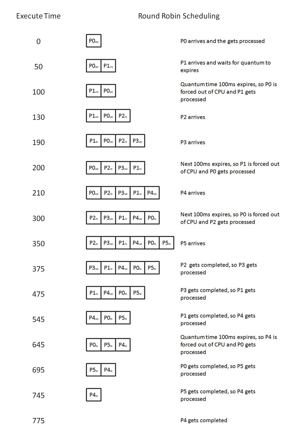 Time quantum allocation in OS (Image: Coolcoder, CC BY-SA 3.0, via Wikimedia Commons)
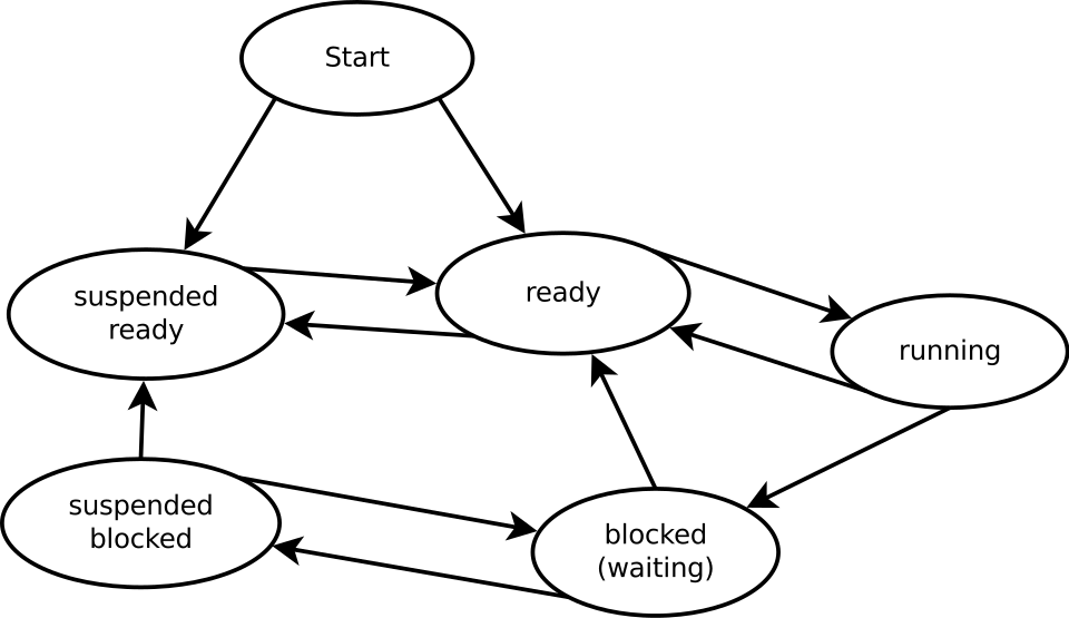 Ready, Running, Waiting transitions (Image: The SVG code is valid. This diagram was created with Dia by , FAL, via Wikimedia Commons)
Based on the TU BCA syllabus for Operating System (CACS251), unit 3.
Discussion
Loading…