Image Restoration & Filtering: Noise Removal, Deconvolution & Frequency-Domain Techniques

TAKEAWAYS:

• Image restoration reverses known degradation (blur, noise) using inverse models, while enhancement improves subjective quality without modeling the degradation process.
• Wiener filtering balances noise suppression and detail preservation by estimating the degradation function and noise statistics.
• Low-pass filters (e.g., Butterworth) smooth images by attenuating high frequencies, but can blur edges; high-pass filters sharpen edges by amplifying high frequencies.
• Frequency-domain filtering (via FFT) lets you design filters in the Fourier space for tasks like removing periodic noise or enhancing textures.
• Deconvolution (e.g., inverse filtering, constrained least squares) recovers the original image from a blurred version, but is sensitive to noise.
• Real-world tradeoffs: Restoration requires knowing the degradation model; enhancement does not, but may introduce artifacts.

1. Image Degradation and Restoration: The Core Problem

What is Image Restoration?

Key Degradation Models:

1. Noise: Random variations in pixel values (e.g., Gaussian noise, salt-and-pepper noise).
2. Blur: Loss of sharpness due to motion, defocus, or atmospheric turbulence.
3. Geometric Distortions: Warping or misalignment (e.g., lens distortion).

Mathematical Model: The observed image $g(x,y)$ is related to the original $f(x,y)$ by: $$g(x,y)=H\{f(x,y)\}+n(x,y)$$ where:

• $H$: Degradation function (e.g., blur kernel).
• $n(x,y)$: Noise (additive or multiplicative).

Goal: Estimate $f(x,y)$ from $g(x,y)$, $H$, and $n(x,y)$.

Visual: Degradation Pipeline

flowchart LR
    A["Original Image \( f(x,y) \)"] -->|"Degradation Function  H "| B["Degraded Image \( g(x,y) \)"]
    B -->|"Noise  n(x,y) "| C["Observed Image (Corrupted)"]
    C -->|"Restoration Algorithm"| D["Restored Image \( \hat{f}(x,y) \)"]

Worked Example: Motion Blur Restoration

Suppose an image is blurred by a horizontal motion kernel $H$: $$H=\frac{1}{5}\left[\begin{array}{ccccc}1& 1& 1& 1& 1\end{array}\right]$$ and the observed image $g$ is: $$g=\left[\begin{array}{ccccc}100& 105& 110& 105& 100\\ 110& 115& 120& 115& 110\\ 120& 125& 130& 125& 120\end{array}\right]$$ Step 1: Assume the original image $f$ is constant (for simplicity). The blur equation becomes: $$g(x,y)=\frac{1}{5}\sum _{i=-2}^{2}f(x+i,y)$$ Step 2: Solve for $f$. For the center pixel $(1,1)$: $$115=\frac{1}{5}(f(1,1)+f(0,1)+f(2,1)+f(3,1)+f(4,1))$$ If $f$ is constant ($f(x,y)=c$): $$115=c⟹c=115$$ Step 3: The restored image is $\hat{f}=115$ (a flat image). In reality, $f$ is not constant, so we need deconvolution.

2. Restoration Techniques

A. Inverse Filtering

Idea: Multiply the Fourier transform of $g$ by the inverse of $H$ to recover $f$: $$F\{\hat{f}\}=\frac{G(u,v)}{H(u,v)}$$ Problem: Amplifies high-frequency noise where $|H(u,v)|$ is small.

Worked Example: Given $H(u,v)=e^{-(u^2+v^2)/20}$ (Gaussian blur), and $G(u,v)$ is the Fourier transform of $g$, compute $\hat{F}(u,v)$: $$\hat{F}(u,v)=\frac{G(u,v)}{e^{-(u^2+v^2)/20}}$$ Visual: Plot $|H(u,v)|$ and $|\hat{F}(u,v)|$ to see noise amplification.

graph TD
    A["\( G(u,v) \)"] -->|"Divide by  H(u,v) "| B["\( \hat{F}(u,v) \)"]
    B -->|"IFFT"| C["Restored Image \( \hat{f} \)"]

B. Wiener Filtering

Idea: A statistical approach that minimizes the mean square error between $\hat{f}$ and $f$. It uses:

• $H(u,v)$: Degradation function in Fourier space.
• $N_0$: Noise power spectrum (assumed constant).
• $S_f(u,v)$: Power spectrum of the original image.

Wiener Filter Formula: $$H_{\text{wiener}}(u,v)=\frac{H^{\ast }(u,v)}{|H(u,v){|}^2+\frac{N_0}{S_f(u,v)}}$$ where $H^{\ast }$ is the complex conjugate of $H$.

Advantages:

• Reduces noise amplification.
• Works well when $H$ and $N_0$ are known.

Disadvantages:

• Requires prior knowledge of $S_f(u,v)$ (often estimated).
• Computationally intensive.

C. Constrained Least Squares (Regularized Inverse Filtering)

Idea: Add a regularization term to stabilize inverse filtering: $$\hat{F}(u,v)=\frac{H^{\ast }(u,v)}{|H(u,v){|}^2+\gamma }$$ where $\gamma$ controls the tradeoff between noise suppression and detail preservation.

Worked Example: For $\gamma =0.1$, compute $\hat{F}(u,v)$ for the Gaussian blur example above. Compare with inverse filtering.

D. Deconvolution via Iterative Methods

Idea: Solve the linear system $g=H\cdot f+n$ iteratively (e.g., Landweber iteration): $$f_{k+1}=f_k+\mu H^T(g-H{f}_k)$$ where $\mu$ is a step size.

Advantages:

• Works for large blur kernels.
• Can incorporate constraints (e.g., non-negativity of pixel values).

Disadvantages:

• Slow convergence.
• Requires tuning $\mu$.

3. Frequency-Domain Filtering

Why Fourier Domain?

• Separation of frequencies: Low frequencies = smooth regions; high frequencies = edges/textures.
• Efficient computation: FFT reduces filtering time from $O(N^2)$ to $O(N\log N)$.

Key Filters

Visual: Frequency Responses

graph TD
    A["Low-Pass Filter"] -->|"Attenuates high  D(u,v) "| B["Smooth Image"]
    C["High-Pass Filter"] -->|"Attenuates low  D(u,v) "| D["Edge-Enhanced Image"]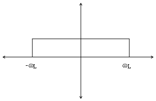

Circular passband in Fourier space. (Image: Public domain, via Wikimedia Commons)

Worked Example: Butterworth Low-Pass Filter

Given:

• Cutoff frequency $D_0=50$ (for a 256×256 image).
• Order $n=2$.

Compute the filter for $(u,v)=(30,40)$: $$D(u,v)=\sqrt{u^2+v^2}=50$$ $$H(u,v)=\frac{1}{1+(50/50{)}^4}=\frac{1}{2}$$ Interpretation: The frequency at $(30,40)$ is attenuated by 50% (3 dB reduction).

4. Spatial-Domain Filtering

Linear Filters (Convolution)

Idea: Apply a kernel $K$ to $g$ to produce $\hat{f}$: $$\hat{f}(x,y)=\sum _{s=-a}^a\sum _{t=-b}^{b}g(x+s,y+t)\cdot K(s,t)$$

Common Kernels:

Worked Example: Noise Removal with Mean Filter Given a noisy image: $$g=\left[\begin{array}{ccc}50& 52& 48\\ 55& 49& 51\\ 53& 50& 54\end{array}\right]$$ Apply the mean filter to the center pixel $(1,1)$: $$\hat{f}(1,1)=\frac{50+52+48+55+49+51+53+50+54}{9}=51$$

Nonlinear Filters

Idea: Replace pixel values based on statistical properties of the neighborhood (e.g., median).

Median Filter:

• Replaces $g(x,y)$ with the median of its neighbors.
• Effective against salt-and-pepper noise.

Worked Example: For the same $g$ above, the median of the 9 pixels is 51 (same as mean here, but differs for impulse noise).

5. Real-World Applications

In Nepal

1. eSewa’s ID Verification:

   • Problem: Scanned ID photos often suffer from blur (motion) and noise (low-light scanning).
   • Solution: Wiener filtering to restore sharpness while reducing noise before OCR (text extraction).
   • Example: A blurred NID card image is restored using a known blur kernel (e.g., Gaussian) and estimated noise variance.

2. Ncell’s Photo-Based Services:

   • Problem: Customer-uploaded photos (e.g., for SIM registration) may have low contrast or camera shake blur.
   • Solution: Adaptive high-pass filtering to enhance edges (e.g., face contours) before facial recognition.

3. NTC’s Traffic Monitoring:

   • Problem: CCTV footage of traffic signals is often noisy (poor lighting) or motion-blurred (vehicles).
   • Solution: Constrained least-squares deconvolution to recover license plates for automated toll systems.

Global Examples

1. Google Photos’ "Magic Eraser":

   • Uses morphological operations + frequency-domain filtering to remove objects (e.g., power lines) from photos.
   • Key Idea: Combines low-pass filtering (to smooth the background) with edge-preserving techniques.

2. WhatsApp’s Sticker Maker:

   • Applies Gaussian blur + adaptive thresholding to create smooth, cartoon-like stickers from photos.
   • Key Idea: Spatial-domain filtering to reduce texture while preserving outlines.

3. Medical Imaging (e.g., MRI Scans):

   • Problem: MRI images suffer from Gaussian noise and motion artifacts.
   • Solution: Wiener filtering to restore diagnostic features (e.g., tumors) while suppressing noise.

6. Comparison: Restoration vs. Enhancement

7. Exam Tips

1. Define Key Terms Precisely:

   • Ideal Low-Pass Filter: A filter with a rectangular frequency response (passes frequencies $D(u,v)\le D_0$, blocks others).
   • Wiener Filter: A statistical filter that minimizes MSE by incorporating noise and signal power spectra.
   • Deconvolution: The process of removing blur by inverting the degradation function $H$.

2. Mathematical Formulas:

   • Memorize the Wiener filter formula and inverse filtering formula in Fourier space.
   • Know the Butterworth filter equation and how its order $n$ affects the transition band.

3. Practical Scenarios:

   • When to use Wiener vs. Inverse Filtering:
     • Use Wiener if noise is significant and $H$ is unknown.
     • Use Inverse if $H$ is known and noise is negligible.
   • Real-World Tradeoffs:
     • Restoration requires more computation but gives better results if $H$ is accurate.
     • Enhancement is faster but may distort features.

4. Diagrams:

   • Draw the block diagram of a restoration system (input $g$, $H$, noise model, filter, output $\hat{f}$).
   • Sketch frequency responses of low-pass/high-pass filters and label $D_0$.

5. Common Pitfalls:

   • Assuming $H$ is known: Restoration fails without the degradation model.
   • Ignoring noise: Inverse filtering amplifies noise; Wiener filtering mitigates this.
   • Over-filtering: High-pass filters can introduce ringing artifacts; low-pass filters can over-blur.

6. Worked Example Patterns:

   • For Wiener filtering, always show:
     1. The Fourier transform of $g$ and $H$.
     2. The power spectra $S_f$ and $N_0$.
     3. The filtered result in both domains.
   • For spatial filtering, show:
     1. The kernel applied.
     2. The convolution operation on a small patch.
     3. The resulting pixel value.

8. Summary Table of Key Techniques