Operational ResearchUnit 811 min read
Game Theory: Payoff Matrices, Optimal Strategies & Real-World Applications
Unit 8 of Operational Research covers zero-sum and non-zero-sum games, payoff matrices, dominance rules, mixed strategies, maximin/minimax, and saddle points—with real-world ties to business competition, pricing wars, and strategic decision-making.
TAKEAWAYS:
- Game theory models conflict and cooperation between rational decision-makers using payoff matrices and optimal strategies.
- Zero-sum games (one player’s gain = another’s loss) use maximin/minimax and saddle points to find optimal mixed strategies.
- Dominance rules simplify payoff matrices by eliminating dominated strategies (pure or mixed).
- Mixed strategies (probability distributions over actions) often yield better outcomes than pure strategies.
- Applications span business competition (market share), auctions, and negotiations (e.g., eSewa vs. Khalti fees).
- Exam focus: Solve 2×2 games, reduce matrices via dominance, and interpret optimal strategies/values.
1. Introduction to Game Theory
Game theory studies strategic interactions where players’ choices affect outcomes. Key assumptions:
- Players are rational (maximize their payoff).
- Players act simultaneously (unless sequential games are specified).
- Outcomes are deterministic (no randomness unless modeled explicitly).
Types of Games
| Type | Description | Example |
|---|---|---|
| Zero-sum | One player’s gain = another’s loss (sum of payoffs = 0). | Poker, market share battles (Company A vs. B). |
| Non-zero-sum | Payoffs are independent (e.g., both can win or lose). | Climate agreements, prisoner’s dilemma. |
| Cooperative | Players can form binding agreements. | Cartels, joint ventures. |
| Non-cooperative | No communication; players act independently. | Auctions, price wars. |
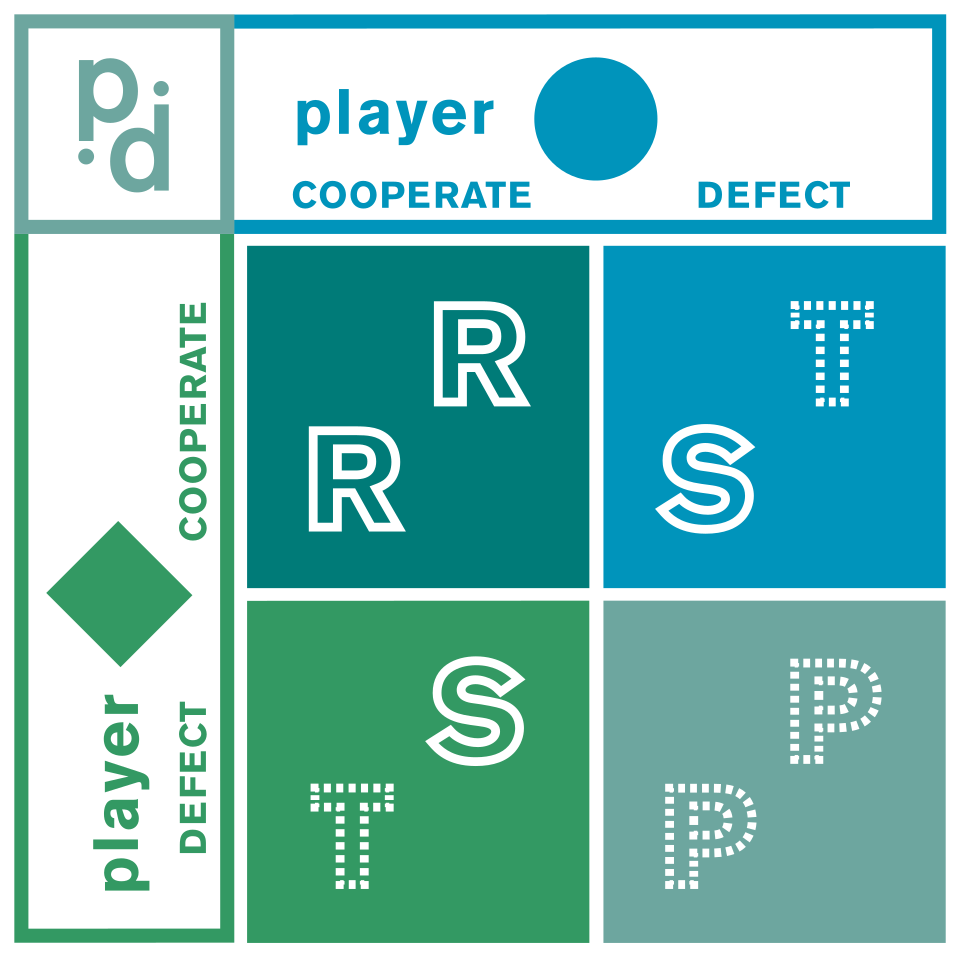 A classic non-zero-sum game showing why cooperation may fail. (Image: Christopher X Jon Jensen (CXJJensen) & Greg Riestenberg, CC BY-SA 3.0, via Wikimedia Commons)
2. Payoff Matrices and Strategies
A payoff matrix represents players’ choices and outcomes. For two players (A and B), it’s structured as:
       B1       B2       B3
A1 [a11, b11] [a12, b12] [a13, b13]
A2 [a21, b21] [a22, b22] [a23, b23]
- Rows: Player A’s strategies.
- Columns: Player B’s strategies.
- Entries:
(A’s payoff, B’s payoff).
Worked Example 1: Market Share Competition
Scenario: Two food manufacturers (Company A and B) compete for market share. The payoff matrix (in % share) is:
       | B: Low Price | B: High Price
A: Low | (30, 20)    | (25, 30)
A: High| (15, 35)    | (20, 25)
Question: Find optimal strategies using maximin/minimax.
Solution:
Player A’s perspective (maximin):
- If B chooses Low: A’s payoffs = 30, 15 → min = 15 (worst case).
- If B chooses High: A’s payoffs = 25, 20 → min = 20.
- Maximin: Choose the maximum of minimums → High Price (20).
Player B’s perspective (minimax):
- If A chooses Low: B’s payoffs = 20, 30 → max = 30 (worst case).
- If A chooses High: B’s payoffs = 35, 25 → max = 35.
- Minimax: Choose the minimum of maximums → Low Price (20).
Outcome: A plays High Price, B plays Low Price → Payoff = (15, 35). Saddle Point: No saddle point exists (no equilibrium where row min = column max).
3. Dominance Rules
Simplify matrices by eliminating dominated strategies (always worse than another option).
Types of Dominance
Pure Dominance:
- A strategy is dominated if another strategy yields higher payoff for all opponent moves.
- Example: In the matrix below, A2 is dominated by A1 (since 4 > 3 and 5 > 2).
A1: [5, 4]
A2: [3, 2]
Mixed Dominance:
- A strategy is mixed-dominated if a probability mix of other strategies always yields a better payoff.
Worked Example 2: Reducing a 3×4 Game
Given Matrix (Player A vs. B):
       B1  B2  B3  B4
A1:    3   2   4   0
A2:    3   4   2   4
A3:    4   2   4   0
A4:    0   4   0   8
Steps:
Eliminate dominated rows:
- Compare A1 and A3: A3 has higher payoffs in B1, B3 → A1 is dominated.
- Compare A2 and A4: A4 has higher payoff in B4 → A2 is not dominated (since A4’s 0 < A2’s 4 in B1).
- Reduced Matrix:
A3: [4, 2, 4, 0]
A4: [0, 4, 0, 8]
Eliminate dominated columns:
- Compare B1 and B3: B3 has higher payoffs for A3 → B1 is dominated.
- Final 2×2 Matrix:
A3: [4, 0]
A4: [0, 8]
4. Mixed Strategies and Optimal Solutions
When no pure strategy dominates, players use probability distributions over actions.
Steps to Solve a 2×2 Zero-Sum Game
- Let Player A choose A1 with probability and A2 with .
- Let Player B choose B1 with probability and B2 with .
- Set expected payoffs equal to the value of the game (V):
- For A:
- For B:
- Solve for .
Worked Example 3: Optimal Strategies for a 2×2 Game
Matrix:
       B1  B2
A1:    3   1
A2:    0   4
Solution:
- Define strategies:
- A: for A1, for A2.
- B: for B1, for B2.
- Expected payoffs:
- For A: → (Equation 1).
- For B: → (Equation 2).
- Solve:
- From Equation 2: .
- Substitute into Equation 1: → .
- At equilibrium, B is indifferent between B1 and B2: → → .
- Substitute into Equation 1: .
- Then .
Optimal Strategies:
- A: Play A1 with 25% probability, A2 with 75%.
- B: Play B1 with 50% probability, B2 with 50%.
- Value of the game (V): 1.5.
5. Saddle Points and Pure Strategy Equilibria
A saddle point is a payoff where:
- It is the minimum in its row (for Player A).
- It is the maximum in its column (for Player B).
Example:
       B1  B2
A1:    2   3
A2:    1   4
- Saddle point: 2 (A1, B1).
- Row min for A1 = 2, Row min for A2 = 1 → 2 is max of mins.
- Column max for B1 = 2, Column max for B2 = 4 → 2 is min of maxes.
If a saddle point exists, it is the optimal pure strategy.
6. Non-Zero-Sum Games: Nash Equilibrium
In non-zero-sum games, players may cooperate or compete. A Nash Equilibrium occurs when no player can benefit by unilaterally changing strategy.
stateDiagram-v2
  [*] --> A: Low
  [*] --> A: High
  A: Low --> B: Low : (3, 3)
  A: Low --> B: High : (0, 5)
  A: High --> B: Low : (5, 0)
  A: High --> B: High : (3, 3)
  note right of B: High
    Nash Equilibrium: (A: High, B: High)
    Both players earn 3, no incentive to deviate.
Prisoner's Dilemma payoff matrix (non-zero-sum Nash Equilibrium).Example: Prisoner’s Dilemma
       | B: Cooperate | B: Defect
A: C   | (-1, -1)    | (-3, 0)
A: D   | (0, -3)     | (-2, -2)
- Nash Equilibrium: (Defect, Defect) → Both defect, even though (Cooperate, Cooperate) is better.
In the Real World
eSewa vs. Khalti (Payment Wars)
- Game Type: Non-zero-sum (both can gain or lose users).
- Strategies:
- Discounts: eSewa offers 5% cashback; Khalti matches.
- Partnerships: Both partner with Daraz for seamless checkout.
- Outcome: Mixed strategies where neither dominates permanently.
Nepal Telecom (NTC) vs. Ncell (Pricing Wars)
- Game Type: Zero-sum (market share gain = competitor’s loss).
- Payoff Matrix:
NTC: Low Price | Ncell: Low Price → (30% share, 20% share) NTC: Low Price | Ncell: High Price → (35% share, 15% share) - Optimal Strategy: NTC uses mixed pricing (sometimes discounts, sometimes premium bundles) to avoid pure dominance.
Daraz vs. Amazon Nepal (Inventory Games)
- Game Type: Sequential (Daraz moves first with pricing; Amazon responds).
- Application: Queuing theory (inventory management) + game theory (price wars).
- Real Scenario: Daraz reduces prices → Amazon matches → Both lose profit but gain users.
Exam Tip
- For payoff matrices:
- Always check for dominance first to reduce the matrix.
- If no saddle point, solve using mixed strategies (set expected payoffs equal).
- Zero-sum vs. non-zero-sum:
- Zero-sum: Use maximin/minimax or mixed strategies.
- Non-zero-sum: Look for Nash Equilibrium.
- Common Pitfalls:
- Forgetting to label payoffs (A’s payoff first, then B’s).
- Misapplying dominance (e.g., not checking all columns/rows).
- Incorrectly setting up expected value equations.
- Past Exam Patterns:
- 2023 TU: Solve a 3×4 game using dominance → reduced to 2×2 → find mixed strategies.
- 2022 PU: Define game theory, assumptions, and business importance (4 marks).
- 2021 NEB: Reduce a game to 2×2 and find optimal strategies (10 marks).
Visual Summary of Key Concepts:
flowchart TD
    A["Game Theory"] --> B["Zero-Sum Games"]
    A --> C["Non-Zero-Sum Games"]
    B --> D["Payoff Matrix"]
    B --> E["Dominance Rules"]
    B --> F["Mixed Strategies"]
    B --> G["Saddle Point"]
    C --> H["Nash Equilibrium"]
    D --> I["Maximin/Minimax"]
    F --> J["Probability Distributions"]
    G --> K["Pure Strategy Equilibrium"]
    H --> L["Prisoner's Dilemma"]
In the real world
eSewa vs. Khalti fee wars: This is a zero-sum game where each company (Player A and B) sets transaction fees (Low/High) to maximize their own revenue. The payoff matrix from Section 2 directly models their strategic choices, with optimal strategies derived via maximin/minimax rules. If one lowers fees (Low Price), the other may retaliate (High Price), leading to a Nash Equilibrium where both earn moderate profits (e.g., (20, 25) in the example).
Nepali mobile operators (Ncell, NTC): The Prisoner’s Dilemma applies to their 4G/5G price wars. If both invest heavily (High Price), they lose customers to cheaper rivals (Low Price). The Nash Equilibrium here is mutual underinvestment (both choose Low Price), harming long-term network quality—a classic non-zero-sum outcome.
NEPSE stock trading: Investors use mixed strategies (probability distributions over buy/sell actions) to hedge risks. For example, a trader might allocate 75% to stocks and 25% to bonds (like Player A’s optimal strategy in Worked Example 3) to balance gains and losses, mirroring game-theoretic optimal solutions.
Based on the TU BCA syllabus for Operational Research (CAOR451), unit 8.
Discussion
Loading…