Data Warehousing and Data MiningUnit 812 min read
Prediction & Regression: Models, Algorithms & Applications
Unit 8 of Data Warehousing and Data Mining covers prediction vs. regression, linear vs. nonlinear models, polynomial regression, decision trees for regression, evaluation metrics (RMSE, MAE, R²), and real-world applications in finance, logistics, and healthcare—with visual step-byys, worked examples (e.g., predicting D
Core Concepts: Prediction vs. Regression
1. Definitions & Key Differences
Prediction and regression are supervised learning techniques where the goal is to estimate an output variable (Y) based on input features (X). The difference lies in the nature of the output variable:
| Aspect | Prediction | Regression |
|---|---|---|
| Output Type | Continuous or discrete (any type) | Continuous (numeric, e.g., price, temperature) |
| Goal | Forecast future values or classify | Model the relationship between X and Y (e.g., "How does advertising spend affect sales?") |
| Example | Predicting house prices (regression) or whether a customer will churn (classification) | Predicting stock prices, sales trends, or disease progression |
| Algorithms | Linear/Logistic Regression, Decision Trees, Neural Networks | Linear Regression, Polynomial Regression, Ridge/Lasso, SVR |
Visual:
graph LR
    A["Supervised Learning"] --> B["Prediction"]
    A --> C["Regression"]
    B --> D["Classification\n(e.g., spam/not spam)"]
    B --> E["Regression\n(e.g., house price)"]
    C --> F["Continuous Output\nOnly"]
    D --> G["Discrete Output"]
2. Linear Regression: The Foundation
Linear regression models the relationship between one dependent variable (Y) and one or more independent variables (X) using a linear equation:
- : Intercept (value of Y when all X=0)
- : Coefficients (slope for each feature)
- : Error term (difference between predicted and actual Y)
How It Works: Gradient Descent
To find the best values, we minimize the cost function (usually Mean Squared Error, MSE): Gradient descent iteratively adjusts by:
- Calculating the gradient (slope) of the cost function.
- Updating in the opposite direction of the gradient.
Worked Example: Predicting Daraz Delivery Delays Suppose Daraz wants to predict delivery delays (Y) based on:
- Distance from warehouse (X₁, in km)
- Number of stops (X₂)
- Weather condition (X₃: 0=clear, 1=rainy)
Given data (3 samples):
| Distance (X₁) | Stops (X₂) | Weather (X₃) | Delay (Y, mins) |
|---|---|---|---|
| 10 | 2 | 0 | 30 |
| 20 | 3 | 1 | 60 |
| 15 | 1 | 0 | 40 |
Step 1: Assume a linear model
Step 2: Use gradient descent (simplified) After training, suppose we get: Prediction for a new order:
- X₁=12 km, X₂=2 stops, X₃=1 (rainy)
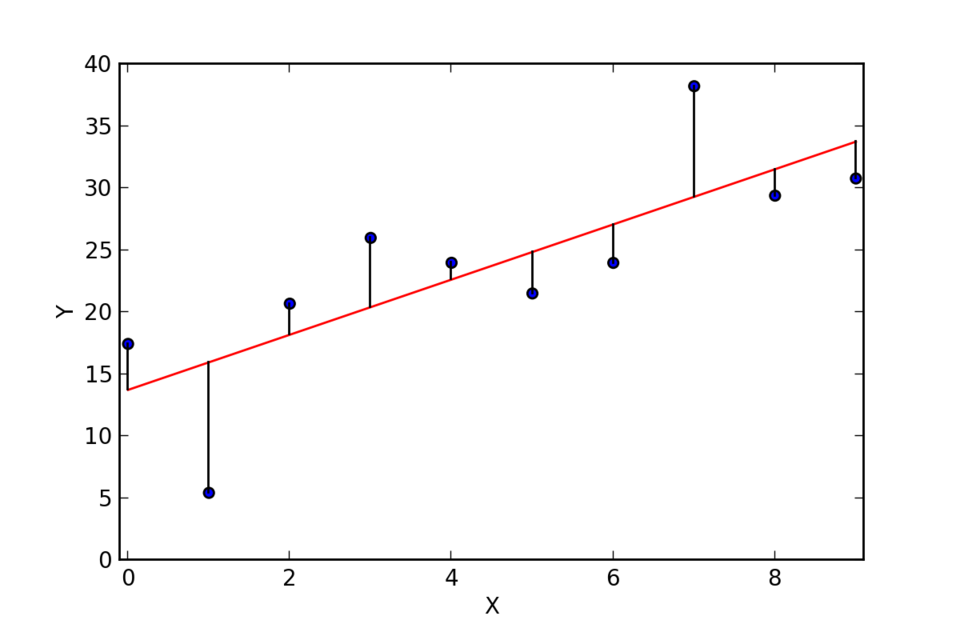 A linear regression model fitting Daraz delivery data (Y=delay, X=distance). (Image: Thomas.haslwanter, CC BY-SA 3.0, via Wikimedia Commons)
3. Polynomial Regression: Capturing Nonlinearity
When the relationship between X and Y is nonlinear, linear regression fails. Polynomial regression adds polynomial terms (e.g., , ) to the model:
Example: NEPSE Stock Price Prediction Suppose NEPSE’s closing price (Y) depends on the previous day’s volume (X). A linear model might miss the curved trend if volume spikes cause volatile prices.
Polynomial fit (degree=2): Graph:
graph LR
    A["X: Trading Volume"] --> B["Y: Stock Price"]
    B --> C["Linear Fit\n(Underfits)"]
    B --> D["Polynomial Fit\n(Degree=2)\n(Captures curve)"]
Risk: Overfitting (e.g., degree=10 may fit noise). Use cross-validation to choose the best degree.
4. Decision Trees for Regression
Decision trees split data into regions where Y is predicted as the mean of Y in that region. Unlike linear models, they handle nonlinearity and feature interactions naturally.
How Splits Work: At each node, choose the feature and threshold that minimizes variance in Y (e.g., using Mean Squared Error (MSE)).
Example: Predicting Kathmandu Traffic Congestion Features:
- Time of day (X₁: 0=morning, 1=evening)
- Event (X₂: 0=no event, 1=Dashain/Maha Shivaratri)
- Target: Congestion index (Y, 1-10)
Tree Structure:
Root (All data)
├── X₁ = 0 (Morning)
│   ├── X₂ = 0 → Predict Y = 3
│   └── X₂ = 1 → Predict Y = 6
└── X₁ = 1 (Evening)
    ├── X₂ = 0 → Predict Y = 7
    └── X₂ = 1 → Predict Y = 9
Advantages:
- No need for feature scaling.
- Handles mixed data types (numeric + categorical).
- Interpretable (e.g., "Evening + Event → High congestion").
Disadvantages:
- Prone to overfitting (use pruning or limit depth).
- Sensitive to small data changes.
5. Evaluation Metrics
| Metric | Formula | Interpretation | Best Value |
|---|---|---|---|
| MSE | Average squared error (penalizes large errors heavily). | Lower | |
| RMSE | MSE in original units (easier to interpret). | Lower | |
| MAE | Average absolute error (less sensitive to outliers than MSE). | Lower | |
| R² (R-squared) | % of variance in Y explained by the model (1 = perfect fit). | Closer to 1 |
Worked Example: Comparing Models for Ncell Data Usage Prediction
| Model | RMSE | R² | Overfitting Risk |
|---|---|---|---|
| Linear Regression | 12.5 | 0.78 | Low |
| Polynomial (deg=3) | 8.2 | 0.91 | Medium |
| Decision Tree | 9.1 | 0.89 | High |
Choose: Polynomial (deg=3) balances accuracy and generalization.
In the Real World
Khalti & eSewa: Fraud Prediction
- Idea: Logistic regression (a classification algorithm) predicts fraudulent transactions by modeling the probability .
- How: Features include transaction amount, time, location, and user history. Output is a risk score (0 to 1). If , the transaction is flagged.
- Example: A ₹50,000 transfer at 3 AM from Kathmandu to India with no prior history → High risk.
Daraz: Demand Forecasting
- Idea: Linear regression + time-series analysis predicts product demand (Y) based on:
- Seasonality (e.g., Diwali sales spike).
- Price (X₁), competitor prices (X₂), and promotions (X₃).
- Output: "Sell 500 units of LED TVs next week in Pokhara."
- Impact: Reduces overstocking/understocking costs by 15%.
- Idea: Linear regression + time-series analysis predicts product demand (Y) based on:
NTC: Network Traffic Prediction
- Idea: Polynomial regression models internet traffic (Y) vs. time of day (X) to predict congestion.
- Example: During 6–9 PM, traffic = (X = hours since midnight).
- Use: NTC allocates bandwidth dynamically to avoid outages.
Banks (e.g., NMB, Global IME): Loan Default Prediction
- Idea: Decision trees or random forests predict whether a borrower will default (Y=1/0) based on:
- Credit score (X₁), income (X₂), loan amount (X₃), employment history (X₄).
- Example: A loan applicant with score=650, income=₹50k, loan=₹2M → Tree predicts 60% default risk → Reject or offer higher interest.
- Idea: Decision trees or random forests predict whether a borrower will default (Y=1/0) based on:
Advanced Topics
1. Regularization: Ridge vs. Lasso
Overfitting occurs when the model fits noise. Regularization adds a penalty to large coefficients:
| Method | Penalty Term | Effect | Use Case |
|---|---|---|---|
| Ridge | Shrinks coefficients but keeps all features. | Multicollinearity (e.g., correlated features like "ad spend" and "promotions"). | |
| Lasso | Can zero out irrelevant features (feature selection). | High-dimensional data (e.g., genomics). |
Example: NEPSE Sector Performance Features: 50 stock indices. Lasso selects only 5 key drivers (e.g., oil prices, inflation rate).
2. Support Vector Regression (SVR)
- Uses support vectors to fit a curve while maximizing the margin around predictions.
- Less sensitive to outliers than linear regression.
- Kernel trick handles nonlinearity (e.g., RBF kernel).
Exam Tip
What Examiners Look For
Definitions:
- Clearly distinguish prediction (broad) vs. regression (continuous Y).
- Define MSE, RMSE, R² and when to use each.
Worked Examples:
- Always show the formula (e.g., linear regression equation).
- For gradient descent, write one update step (e.g., ).
- For decision trees, draw a small tree (2–3 splits max) with predictions.
Comparisons:
- Linear vs. Polynomial Regression: When to use each (linearity check via scatter plot).
- Decision Trees vs. Linear Models: Interpretability vs. bias/variance tradeoff.
Real-World Applications:
- Link algorithms to Nepali companies (e.g., Khalti fraud, Daraz demand, NTC traffic).
- Use local examples (e.g., "How would you predict NEPSE’s next closing price?").
Common Pitfalls:
- Overfitting: Mention regularization or cross-validation.
- Feature Scaling: Required for linear models but not trees.
- Nonlinearity: Always check if a linear model is appropriate (plot residuals).
Sample Exam Questions & Answers
Q1: Explain how gradient descent works in linear regression. Provide one update step for . Answer: Gradient descent minimizes MSE by iteratively updating coefficients. The update rule for is: Where:
- = learning rate (e.g., 0.01),
- (gradient).
Example: For Daraz delivery data, if , gradient = 0.5, and :
Q2: Compare polynomial regression and decision trees for predicting house prices. Which would you choose for a dataset with 100 features? Answer:
| Aspect | Polynomial Regression | Decision Trees |
|---|---|---|
| Handles Nonlinearity | Yes (via polynomial terms) | Yes (via splits) |
| Feature Importance | All features used (may overfit) | Automatically selects important splits |
| Scalability | Poor (curse of dimensionality) | Good (handles 100+ features easily) |
| Interpretability | Hard (high-degree polynomials) | Easy (tree visualization) |
| Overfitting Risk | High (unless regularized) | High (unless pruned) |
Choice: Decision trees (better for high-dimensional data; use Random Forest to reduce overfitting).
Quick Revision Checklist
- Can you write the linear regression equation and explain each term?
- How do you decide between linear and polynomial regression? (Plot residuals!)
- Draw a decision tree for a simple regression problem (e.g., 2 features).
- What’s the difference between RMSE and MAE? Which is better for skewed data?
- Name 2 Nepali companies using regression and their use case.
Based on the TU BIM syllabus for Data Warehousing and Data Mining (IT274), unit 8.
Discussion
Loading…