Unit 10 – Index Numbers & Time Series Analysis (Basic Concepts)

Introduction to Index Numbers

An index number is a dimensionless ratio that expresses the relative change in a variable (price, quantity, value) between two periods.

• Base year $B$: the period against which all other periods are compared.
• Index value $I_t$ for period $t$ is usually expressed as a percentage of the base year (100).

$$I_t=\frac{S_t}{S_B}\times 100$$

where $S_t$ and $S_B$ are the summed values (prices, quantities, etc.) in period $t$ and the base year, respectively.

Types of Index Numbers

Common Price Indices

1. Laspeyres Index (fixed base‑year quantities)
   $$L_t=\frac{{\sum }_i{P}_{i,t}{Q}_{i,B}}{{\sum }_i{P}_{i,B}{Q}_{i,B}}\times 100$$
2. Paasche Index (fixed current‑year quantities)
   $$P_t=\frac{{\sum }_i{P}_{i,t}{Q}_{i,t}}{{\sum }_i{P}_{i,B}{Q}_{i,t}}\times 100$$
3. Fisher Index (geometric mean of Laspeyres and Paasche)
   $$F_t=\sqrt{L_t\times P_t}$$
4. Chain Index (sequential linking)
   $$C_t=\prod _{k=1}^t\frac{S_k}{S_{k-1}}\times 100$$

Worked Example – Laspeyres Price Index

Suppose a basket contains three goods: rice, wheat, and cooking oil.

Step 1: Compute base‑year total value
$$S_B=30\times 100+25\times 80+20\times 50=3000+2000+1000=6000$$

Step 2: Compute current‑year total value using base‑year quantities
$$S_t=35\times 100+27\times 80+22\times 50=3500+2160+1100=6760$$

Step 3: Laspeyres index
$$L_t=\frac{6760}{6000}\times 100=112.67$$

Interpretation: Prices have risen by 12.67 % relative to the base year.

Index Number Comparison Table

Time‑Series Analysis – Basic Concepts

A time series is a sequence of observations recorded at successive equally spaced time intervals.

Components of a Time Series

1. Trend (T) – long‑term direction (upward, downward, or stationary).
2. Seasonality (S) – regular pattern repeating within a fixed period (e.g., monthly sales peaks).
3. Cyclical (C) – long‑term oscillations not fixed to a calendar period.
4. Irregular (I) – random noise or unexpected shocks.

Mathematically, for an additive model:
$$Y_t=T_t+S_t+C_t+I_t$$ For a multiplicative model:
$$Y_t=T_t\times S_t\times C_t\times I_t$$

Visualising a Time Series

The blue line shows observed sales, the red line the estimated trend, and the green line the seasonal component.

Decomposition Methods

• Additive decomposition is appropriate when seasonal fluctuations are roughly constant over time.
• Multiplicative decomposition is used when seasonal variations change proportionally with the level of the series.

Decomposition Process (Mermaid)

flowchart TD
    "Observed Series" --> "Estimate Trend (Moving Avg)"
    "Observed Series" --> "Detrend (Subtract Trend)"
    "Detrend" --> "Estimate Seasonal (Average of Detrended)"
    "Detrend" --> "Detrend Seasonal (Subtract Seasonal)"
    "Detrend Seasonal" --> "Irregular Component"

Forecasting Techniques

1. Moving Average (MA)

A simple method that smooths short‑term fluctuations by averaging a fixed number of past observations.

$$M{A}_t=\frac{1}{k}\sum _{i=0}^{k-1}{Y}_{t-i}$$

Worked Example – 3‑Month MA

2. Exponential Smoothing (ES)

Weights all past observations but assigns exponentially decreasing weights to older data.

$$S_t=\alpha Y_t+(1-\alpha )S_{t-1}$$

where $0<\alpha <1$ is the smoothing constant.

Worked Example – $\alpha =0.5$

In the Real World

Concrete Example – Daraz Price Index
Daraz monitors the price of a flagship smartphone.

• Base year price: Rs 30,000 (January 2023).
• Current price: Rs 32,000 (January 2024).
  Using a Fisher index (assuming equal weights for simplicity):
  $$F=\sqrt{\frac{32,000}{30,000}\times \frac{30,000}{32,000}}=1.0$$ The index remains 100, indicating no net price change when considering both price and quantity adjustments. This informs Daraz’s dynamic pricing strategy.

Exam Tip

1. Index Calculations – Practice computing Laspeyres, Paasche, Fisher, and chain indices. Memorise the formulas and the role of base‑year quantities.
2. Time‑Series Decomposition – Be able to identify trend, seasonal, cyclical, and irregular components from a given plot. Know when to use additive vs. multiplicative models.
3. Forecasting Methods – Understand the difference between moving averages and exponential smoothing, and when each is appropriate.
4. Interpretation – Exams often ask for interpretation of index values or forecasted figures; practice explaining what a 112.5 index or a 3‑month MA of 17.7 means in context.
5. Worked Example – Include all steps, show intermediate calculations, and label your figures clearly.

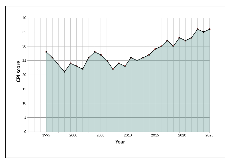Consumer Price Index trend in Nepal (Image: Amitchell125, CC BY 4.0, via Wikimedia Commons)