Measures of Central Tendency – Mean, Median, Mode & Their Relationships

1. Definitions

Grouped data – observations are presented in class intervals.

• Mean (grouped): $\bar{x}=\frac{\sum f_i{m}_i}{\sum f_i}$ where $f_i$ = frequency, $m_i$ = class midpoint.
• Median (grouped): $M=L+\left(\frac{\frac{N}{2}-c_f}{f_m}\right)h$ where $L$ = lower limit of median class, $c_f$ = cumulative frequency before median class, $f_m$ = frequency of median class, $h$ = class width.
• Mode (grouped): $Mo=L+\left(\frac{f_m-f_{m-1}}{(f_m-f_{m-1})+(f_m-f_{m+1})}\right)h$ where $f_{m-1},f_{m+1}$ are frequencies of classes adjacent to modal class.

2. Worked Example – Ungrouped Data

Problem:
Monthly income (Rs.) of 20 families:
$45,55,55,60,70,70,70,80,85,90,90,95,100,100,100,110,115,120,130,150$

1. Find mean, median and mode.
2. Decide which measure best represents the central tendency.

Solution Steps

1. Mean
   $$\bar{x}=\frac{45+55+55+60+70+70+70+80+85+90+90+95+100+100+100+110+115+120+130+150}{20}$$
   $$\bar{x}=\frac{1765}{20}=88.25\text{Rs.}$$

2. Median – arrange (already sorted). $n=20$ (even) → median is average of 10th and 11th values.
   10th = 90, 11th = 90 → $M=\frac{90+90}{2}=90$ Rs.

3. Mode – frequency table:

Both 70 and 100 appear three times → bimodal: modes = 70 Rs. and 100 Rs.

4. Choice of measure – The distribution is slightly right‑skewed (high income 150). The median (90 Rs.) is less affected by the outlier than the mean (88.25 Rs.) and lies between the two modes. For reporting a typical family income, median is preferred.

3. Worked Example – Grouped Data

Problem:
The following grouped data show the number of customers visiting a café per day.

Compute mean, median and mode.

Solution

1. Class mid‑points $m_i$: 4.5, 14.5, 24.5, 34.5, 44.5.

2. Mean (grouped)

$$\bar{x}=\frac{\sum f_i{m}_i}{\sum f_i}=\frac{5(4.5)+12(14.5)+20(24.5)+8(34.5)+5(44.5)}{5+12+20+8+5}$$

$$\bar{x}=\frac{22.5+174+490+276+222.5}{50}=\frac{1185}{50}=23.7\text{customers}$$

3. Median (grouped)

Total $N=50$; $N/2=25$. Cumulative frequencies: 5, 17, 37, 45, 50.
Median class = 20‑29 (cumulative before = 17, $f_m=20$).

$$L=20,h=10,c_f=17$$

$$M=20+\left(\frac{25-17}{20}\right)10=20+\left(\frac{8}{20}\right)10=20+4=24\text{customers}$$

4. Mode (grouped)

Modal class = 20‑29 ($f_m=20$). Adjacent frequencies: $f_{m-1}=12$, $f_{m+1}=8$.

$$Mo=20+\left(\frac{20-12}{(20-12)+(20-8)}\right)10=20+\left(\frac{8}{8+12}\right)10=20+\frac{8}{20}\times 10=20+4=24\text{customers}$$

Interpretation: Mean (23.7) ≈ Median (24) ≈ Mode (24) → distribution is approximately symmetric.

4. Comparative Table

5. Coefficient of Variation (CV)

CV expresses dispersion relative to the mean, useful for comparing variability of data measured in different units.

$$\text{CV}=\frac{s}{\bar{x}}\times 100\%$$

Example: Mean = 32, SD = 17 →

$$\text{CV}=\frac{17}{32}\times 100\%=53.125\%$$

A CV > 50 % indicates high relative variability; in business, a product line with CV = 80 % would be considered unstable in demand.

6. Pearson’s Coefficient of Skewness

Two common forms:

1. Based on mean and mode
   $${\text{Skewness}}_1=\frac{\bar{x}-\text{Mo}}{s}$$

2. Based on mean and median
   $${\text{Skewness}}_2=3\frac{\bar{x}-M}{s}$$

Worked Example:
Mean = 25, Mode = 20, SD = 10

$${\text{Skewness}}_1=\frac{25-20}{10}=0.5(\text{positive, right‑skewed})$$

7. Combined (Pooled) Mean

When two independent groups are merged:

$${\bar{x}}_{\text{combined}}=\frac{n_1{\bar{x}}_1+n_2{\bar{x}}_2}{n_1+n_2}$$

Example:
Group A: ${\bar{x}}_A=65$, $n_A=40$
Group B: ${\bar{x}}_B=60$, $n_B=60$

$${\bar{x}}_c=\frac{40(65)+60(60)}{100}=\frac{2600+3600}{100}=62$$

8. Standard Error of the Mean (SEM)

$$\text{SEM}=\frac{s}{\sqrt{n}}$$

When the population size $N$ is finite, apply finite‑population correction (FPC):

$${\text{SEM}}_{\text{FPC}}=\frac{s}{\sqrt{n}}\sqrt{\frac{N-n}{N-1}}$$

Example: $N=1000,n=100,s=10$

$$\text{SEM}=\frac{10}{\sqrt{100}}=1.0$$

$${\text{SEM}}_{\text{FPC}}=1.0\sqrt{\frac{1000-100}{999}}=1.0\sqrt{\frac{900}{999}}\approx 0.95$$

9. Relationships Among Mean, Median, Mode

For moderately skewed distributions:

mindmap
root((Central Tendency Relationships))
    Mean --> "Sensitive to outliers"
    Median --> "Resistant to outliers"
    Mode --> "Most frequent value"
    "Mean, Median, Mode" --> "Mode ≈ 3·Median – 2·Mean"

$$\text{Mode}\approx 3\text{Median}-2\text{Mean}$$

Example: Mean = 30, Median = 28 →

$$\text{Mode}\approx 3(28)-2(30)=84-60=24$$

flowchart LR
    A["Data Set"] --> B["Compute Mean (uses all values)"]
    A --> C["Sort & Find Median (position based)"]
    A --> D["Tabulate Frequencies → Mode (most frequent)"]
    B --> E["Sensitive to outliers"]
    C --> F["Resistant to outliers"]
    D --> G["May be multiple or none"]
    E --> H["Best for symmetric data"]
    F --> I["Best for skewed data"]
    G --> J["Best for categorical data"]

10. In the real world

• eSewa & Khalti (digital wallets) – When displaying the “average transaction value” to merchants, the mean is used because it incorporates every transaction amount, helping merchants forecast cash flow.
• Daraz order queue – The median delivery time is shown on the website (e.g., “Median delivery: 3 days”). This protects customers from a few extremely delayed orders that would inflate the mean.
• NTC mobile data usage – The mode of daily data consumption (e.g., 500 MB) identifies the most common usage tier, guiding the company to design popular data packages.

Worked real‑world tie‑in:
A bank analyses loan applicants’ annual incomes. The data are heavily right‑skewed because a few high‑net‑worth clients earn > Rs 5 million. The bank reports the median income (Rs 850,000) to set a realistic minimum income requirement, rather than the mean (Rs 1.2 million) which would be misleadingly high.

11. Common Pitfalls

In the real world

• eSewa & Khalti – When merchants view the average transaction value on their dashboard, the platform displays the mean of all transactions so that revenue forecasts include every sale.
• Daraz – The site shows “Median delivery time: 3 days” on product pages; the median protects customers from a few unusually long deliveries that would inflate the mean.
• NTC – In its monthly data‑usage report, NTC highlights the mode of daily data consumption (e.g., 500 MB) to design the most popular data‑plan tier.

Exam tip

• Read the data format first – decide whether the question gives raw, grouped, or frequency‑class data; choose the appropriate formulas.
• Always compute the mean first; many other measures (combined mean, CV, skewness) need it.
• For median in grouped data, write down cumulative frequencies; a small arithmetic slip in $c_f$ leads to a wrong answer.
• When the question asks “choose the best measure,” justify with a brief comment on skewness or presence of outliers (e.g., “distribution is right‑skewed; median is less affected by the high‑value outlier”).
• Mark units clearly (Rs., customers, kg) – examiners award marks for correct units.

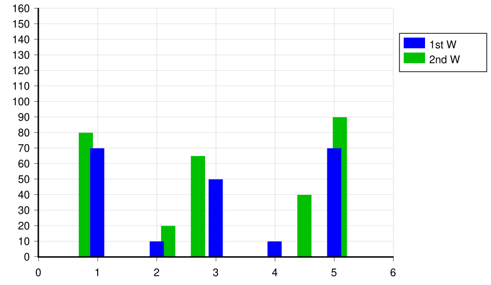Bar chart representing frequency distribution of monthly income (used in the ungrouped data example) (Image: Innesw, CC BY-SA 3.0, via Wikimedia Commons)