Economics for BusinessUnit 513 min read
Theory of Cost: Short-run vs. Long-run, Cost Curves, Economies of Scale
Unit 5 of Economics for Business explains how businesses calculate costs (fixed, variable, total, average, marginal), how cost curves behave in the short run and long run, and why cost structures differ across industries—with real-world examples from Nepalese firms like Ncell and Daraz.
TAKEAWAYS
- Costs are classified into fixed (e.g., rent), variable (e.g., raw materials), and total costs, and their relationships are shown by cost curves.
- Short-run costs (e.g., Ncell’s daily labor costs) are influenced by fixed factors like plant size, while long-run costs (e.g., Daraz’s warehouse expansion) allow all inputs to vary.
- Average cost (AC) and marginal cost (MC) curves intersect at their minimum points, forming the "U-shape" critical for profit maximization.
- Economies of scale (e.g., NTC’s bulk power generation) reduce per-unit costs as output increases, while diseconomies of scale (e.g., Kathmandu traffic congestion) increase costs beyond a certain scale.
- Cost curves (AFC, AVC, AC, MC) determine a firm’s supply curve in competitive markets.
- Break-even analysis (e.g., a local bakery’s sales target) uses cost-volume-profit relationships to find the output level where total revenue equals total cost.
1. Classification of Costs
Costs are the expenses incurred by a business to produce goods or services. They are classified into three primary types:
1.1 Fixed Costs (FC)
- Definition: Costs that do not change with the level of output in the short run. These are incurred even if the firm produces zero units.
- Examples:
- Rent for factory space (e.g., Daraz’s warehouse in Lalitpur).
- Salaries of permanent employees (e.g., Ncell’s customer service staff).
- Insurance premiums (e.g., a local bakery’s shop insurance).
- Key Point: Fixed costs are sunk costs in the short run—they cannot be recovered if the business shuts down temporarily.
1.2 Variable Costs (VC)
- Definition: Costs that vary directly with the level of output. They increase as production rises and decrease as production falls.
- Examples:
- Raw materials (e.g., wheat flour for a bakery).
- Electricity bills (e.g., NTC’s power consumption for a factory).
- Wages for temporary workers (e.g., Pathao’s delivery agents during peak hours).
- Key Point: Variable costs are avoidable in the short run if production stops.
1.3 Total Costs (TC)
- Definition: The sum of fixed costs and variable costs at any given level of output.
- Example: If a local bakery has fixed costs of Rs. 50,000 (rent, salaries) and variable costs of Rs. 20 per loaf, the total cost for 1,000 loaves is:
1.4 Average Costs (AC)
- Definition: The cost per unit of output. It is calculated by dividing total cost by the quantity produced.
- Average Fixed Cost (AFC):
- Average Variable Cost (AVC):
1.5 Marginal Cost (MC)
- Definition: The additional cost incurred by producing one more unit of output. It is calculated as the change in total cost divided by the change in quantity.
- Example: If producing 100 loaves costs Rs. 60,000 and producing 101 loaves costs Rs. 60,020, the marginal cost of the 101st loaf is:
2. Cost Curves in the Short Run
In the short run, at least one factor of production (usually plant capacity) is fixed. The behavior of cost curves in this period is critical for decision-making.
2.1 Shape of Cost Curves
The short-run cost curves exhibit a U-shape due to the law of diminishing marginal returns. Here’s how they behave:
2.2 Key Relationships
AFC Curve:
- Always downward-sloping because fixed costs are spread over a larger number of units as output increases.
- Example: If a factory’s rent is Rs. 100,000, producing 10,000 units makes AFC = Rs. 10/unit, while producing 20,000 units makes AFC = Rs. 5/unit.
AVC Curve:
- Initially decreases due to specialization and efficient use of resources.
- Later increases due to diminishing returns (e.g., overcrowding in a small factory).
- Example: A bakery’s AVC for the first 50 loaves is Rs. 15/loaf, but rises to Rs. 25/loaf for the next 50 due to overtime labor costs.
AC Curve:
- Also U-shaped because it is the sum of AFC (always decreasing) and AVC (U-shaped).
- The minimum point of AC is where MC = AC.
MC Curve:
- U-shaped due to diminishing returns.
- Intersects AC at its minimum point. This is a crucial rule for profit maximization.
- Example: If a firm’s AC is Rs. 30/unit at 100 units and MC rises to Rs. 30 at 101 units, producing beyond 100 units will increase AC.
- FC = Rs. 50,000
- VC at Q=100 = Rs. 20,000 (AVC = Rs. 200/unit)
- VC at Q=200 = Rs. 35,000 (AVC = Rs. 175/unit)
- VC at Q=300 = Rs. 60,000 (AVC = Rs. 200/unit)
3. Long-Run Costs and Economies of Scale
In the long run, all factors of production can be varied. Firms can adjust plant size, technology, and labor to optimize production.
3.1 Long-Run Average Cost (LRAC) Curve
- The LRAC curve is flatter than the short-run AC curve because firms can choose the most efficient plant size for any output level.
- It shows the minimum possible cost of producing any output level when all inputs are variable.
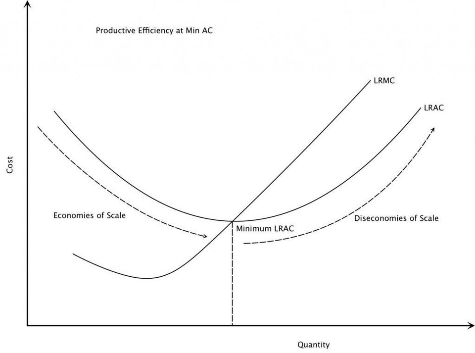 LRAC curve showing economies of scale (downward-sloping), constant returns, and diseconomies (upward-sloping). (Image: District2013, CC BY-SA 4.0, via Wikimedia Commons)
3.2 Economies of Scale
- Definition: Reductions in per-unit costs as output increases due to efficient use of resources, specialization, and bulk purchasing.
- Types:
- Technical Economies: Larger plants use machinery more efficiently (e.g., NTC’s hydropower dams).
- Managerial Economies: Larger firms can afford specialized managers (e.g., Daraz’s supply chain team).
- Financial Economies: Lower interest rates for large loans (e.g., Global IME Bank’s corporate borrowing).
- Marketing Economies: Bulk advertising reduces per-unit cost (e.g., Ncell’s nationwide promotions).
3.3 Diseconomies of Scale
- Definition: Increases in per-unit costs as a firm grows too large, often due to coordination problems, bureaucracy, or inefficiencies.
- Examples:
- Nepal’s Traffic Congestion: Kathmandu’s chaotic traffic increases delivery costs for Pathao and Foodmandu.
- Overstaffing: A bloated corporate hierarchy (e.g., a government office) leads to higher salaries and lower productivity.
- Communication Breakdowns: Large firms like NMB Bank may struggle with slow decision-making.
- Decreasing LRAC (economies of scale) from Q=0 to Q=500.
- Constant LRAC (constant returns to scale) from Q=500 to Q=1,000.
- Increasing LRAC (diseconomies of scale) beyond Q=1,000. Assume:
- At Q=100, LRAC = Rs. 50/unit.
- At Q=500, LRAC = Rs. 30/unit (minimum efficient scale).
- At Q=2,000, LRAC = Rs. 40/unit (due to diseconomies).
4. Cost Curves and Market Supply
Cost curves determine a firm’s supply curve in competitive markets:
- A firm will produce where Price (P) = Marginal Cost (MC) (above AVC).
- The short-run supply curve is the portion of the MC curve above AVC.
- Example: If a firm’s AVC is Rs. 100/unit and MC rises to Rs. 150 at Q=100, it will supply 100 units only if the market price is ≥ Rs. 150.
5. Break-Even Analysis
Break-even analysis determines the minimum sales volume needed to cover all costs (fixed and variable). It is crucial for startups and small businesses.
5.1 Break-Even Point (BEP)
- The point where Total Revenue (TR) = Total Cost (TC).
- At BEP, Profit = 0.
- Formula:
Where:
- = Selling price per unit.
- = Average variable cost per unit.
5.2 Worked Example: Local Bakery
Assume:
- Fixed Costs (FC) = Rs. 30,000/month (rent, salaries).
- Variable Cost per loaf (AVC) = Rs. 20.
- Selling Price per loaf (P) = Rs. 50.
- Calculate BEP:
- Interpretation: The bakery must sell 1,000 loaves/month to cover all costs. Below this, it incurs a loss; above this, it makes a profit.
5.3 Profit and Loss Regions
- Below BEP: Loss = FC + (AVC × Q) – (P × Q).
- At BEP: Profit = 0.
- Above BEP: Profit = (P × Q) – (FC + AVC × Q).
- X-axis: Quantity (loaves).
- Y-axis: Cost and Revenue (Rs.).
- FC line: Horizontal at Rs. 30,000.
- VC line: Upward-sloping (Rs. 20 × Q).
- TC line: FC + VC (upward-sloping).
- TR line: Upward-sloping (Rs. 50 × Q).
- BEP: Where TR = TC at Q=1,000.
In the Real World
Ncell’s Network Expansion:
- Idea Used: Economies of Scale.
- How: Ncell reduces the per-unit cost of providing mobile services by expanding its network infrastructure. Bulk purchasing of spectrum licenses and shared towers lowers its average cost, allowing it to offer cheaper data plans to consumers.
Daraz’s Warehouse Operations:
- Idea Used: Short-run vs. Long-run Costs.
- How: Daraz operates in the short run with fixed warehouse sizes but adjusts variable costs (e.g., hiring seasonal workers during Diwali) to meet demand spikes. In the long run, it builds larger warehouses (e.g., in Chitwan) to achieve economies of scale, reducing shipping costs per order.
Pathao’s Delivery Pricing:
- Idea Used: Marginal Cost and Break-even Analysis.
- How: Pathao sets dynamic pricing based on marginal costs (e.g., surge pricing during peak hours in Thapathali). The break-even point for a delivery agent is calculated by ensuring the fare covers variable costs (fuel, time) plus a portion of fixed costs (bike maintenance, insurance).
Nepal’s Traffic Congestion (NTC and Public Transport):
- Idea Used: Diseconomies of Scale.
- How: Kathmandu’s unplanned urban growth leads to traffic jams, increasing the marginal cost of commuting. Public transport like NTC buses face higher operational costs due to delays, reducing their efficiency and profitability.
Nepal Rastra Bank’s Loan Interest Rates:
- Idea Used: Average Cost and Marginal Cost.
- How: Banks like Global IME set loan interest rates based on their average cost of funds (deposits, borrowing) plus a margin. For small loans (e.g., Rs. 100,000), the marginal cost of processing is high, so interest rates are higher than for bulk corporate loans.
Exam Tip
Diagrams Are Mandatory:
- Always draw short-run cost curves (AFC, AVC, AC, MC) with labels and equilibrium points. Examiners expect you to show:
- AFC always decreasing.
- AVC and AC U-shaped.
- MC intersecting AC at its minimum.
- For long-run costs, sketch the LRAC curve with economies and diseconomies of scale.
- Always draw short-run cost curves (AFC, AVC, AC, MC) with labels and equilibrium points. Examiners expect you to show:
Numerical Problems:
- Practice break-even analysis and cost minimization problems. Use the formula:
- Example: If FC = Rs. 20,000, P = Rs. 100, AVC = Rs. 60, then BEP = 500 units.
Real-World Applications:
- Relate cost theories to Nepalese businesses (e.g., Ncell’s scale economies, Daraz’s fixed costs, Pathao’s marginal costs).
- Discuss diseconomies of scale in contexts like Kathmandu’s traffic or government inefficiencies.
Key Formulas to Memorize:
Common Mistakes to Avoid:
- Confusing short-run and long-run costs: Remember, fixed costs exist only in the short run.
- Ignoring the intersection of MC and AC: Always state that MC cuts AC at its minimum.
- Assuming all cost curves are U-shaped: AFC is always downward-sloping.
Summary Table: Short-Run vs. Long-Run Costs
| Feature | Short Run | Long Run |
|---|---|---|
| Fixed Factors | At least one fixed (e.g., plant size) | All factors variable |
| Cost Curves | AFC, AVC, AC, MC (U-shaped) | LRAC (flatter, shows economies) |
| Diminishing Returns | Applies (e.g., overworked labor) | Does not apply (all inputs adjustable) |
| Example | Ncell’s daily labor costs | Daraz’s warehouse expansion |
| Decision Making | Shutdown rule (P < AVC) | Optimal plant size choice |
Based on the TU BITM syllabus for Economics for Business (ECO206), unit 5.
Discussion
Loading…