Programming with PythonUnit 912 min read
NumPy & Pandas: Arrays, DataFrames & Analysis
Unit 9 of Programming with Python covers NumPy for numerical computing (arrays, operations, broadcasting) and Pandas for data analysis (Series, DataFrames, indexing, merging, time-series). Learn how to clean, transform, and visualize real-world datasets like stock prices or customer transactions.
TAKEAWAYS:
- NumPy arrays are homogeneous, fixed-size, and vectorized for fast math operations (e.g.,
array + 5adds 5 to every element). - Pandas DataFrames combine rows (observations) and columns (features) like a spreadsheet, with built-in methods for filtering, grouping, and aggregation.
- Broadcasting lets NumPy perform operations between arrays of different shapes (e.g., adding a scalar to a 2D array).
- Pandas handles missing data (
NaN) with methods likedropna()orfillna(), and time-series withDatetimeIndex. - Merging/joining DataFrames (
merge(),concat()) is critical for combining datasets (e.g., customer orders + product inventory). - Visualization with
matplotliborseabornturns data into insights (e.g., Daraz’s sales trends or NEPSE stock performance).
1. NumPy: Numerical Computing with Arrays
NumPy (Numerical Python) is a library for fast numerical operations using n-dimensional arrays. Unlike Python lists, NumPy arrays are:
- Homogeneous: All elements must be the same type (e.g.,
int32,float64). - Fixed-size: Resizing requires creating a new array.
- Vectorized: Operations apply to entire arrays without loops (e.g.,
array * 2doubles every element).
Key Concepts
1.1 Creating Arrays
import numpy as np

# From a list
arr1 = np.array([1, 2, 3])  # 1D array
arr2 = np.array([[1, 2], [3, 4]])  # 2D array (matrix)

# Special arrays
zeros = np.zeros((3, 3))  # 3x3 matrix of zeros
ones = np.ones((2, 2))    # 2x2 matrix of ones
identity = np.eye(3)      # 3x3 identity matrix
range_arr = np.arange(0, 10, 2)  # [0, 2, 4, 6, 8]
Visual: 1D vs. 2D Array
1.2 Array Indexing and Slicing
arr = np.array([[1, 2, 3], [4, 5, 6]])

# Access element (row 1, column 2)
print(arr[1, 2])  # Output: 6

# Slice rows 0-1, columns 1-2
print(arr[0:2, 1:3])
# Output: [[2, 3], [5, 6]]
Trace Table: Slicing Steps
| Step | Code | Result |
|---|---|---|
| 1 | arr[0:2, 1:3] |
Selects rows 0 and 1 |
| 2 | Selects columns 1 and 2 | |
| 3 | Returns [[2, 3], [5, 6]] |
1.3 Universal Functions (ufuncs)
NumPy provides element-wise operations without loops:
arr = np.array([1, 4, 9])
print(np.sqrt(arr))  # [1.0, 2.0, 3.0]
print(np.sin(arr))   # [0.8415, -0.7568, 0.4121]
1.4 Broadcasting
Broadcasting allows operations between arrays of different shapes by virtually expanding the smaller array. Rule: Compare shapes from the rightmost dimension:
- If dimensions match or one is
1, the smaller array is stretched. - If neither matches, an error occurs.
Example: Adding a scalar to a 2D array
arr = np.array([[1, 2], [3, 4]])
scalar = 5
result = arr + scalar  # Broadcasts scalar to shape (1,1) -> (2,2)
Visual: Broadcasting Steps
1.5 Real-World Example: Calculating Loan Payments
Banks (e.g., Nabil Bank) use NumPy to compute Equated Monthly Installments (EMI) for loans. The formula for EMI is: where:
- = principal loan amount,
- = monthly interest rate,
- = number of payments.
Code Example:
def calculate_emi(principal, annual_rate, years):
    monthly_rate = annual_rate / 12 / 100
    num_payments = years * 12
    emi = principal * (monthly_rate * (1 + monthly_rate)**num_payments) / ((1 + monthly_rate)**num_payments - 1)
    return emi

# Example: Loan of Rs. 1,000,000 at 8% annual rate for 5 years
emi = calculate_emi(1000000, 8, 5)
print(f"EMI: Rs. {emi:.2f}")  # Output: EMI: Rs. 19,801.64
Trace Table: EMI Calculation
| Variable | Value |
|---|---|
principal |
1,000,000 |
annual_rate |
8 |
monthly_rate |
0.006666... |
num_payments |
60 |
emi |
19,801.64 |
2. Pandas: Data Analysis with DataFrames
Pandas provides DataFrames (2D tables) and Series (1D arrays) for data manipulation. Key features:
- Handling missing data (
NaN). - Filtering, grouping, and aggregation.
- Merging datasets (like SQL joins).
- Time-series analysis.
2.1 Creating DataFrames
import pandas as pd

```figure
{"type":"array","values":[["Name","Age","Salary"],["Ramesh",25,50000],["Sita",30,60000],["Hari",22,45000]],"caption":"Example DataFrame from list of lists"}
From a dictionary
data = { "Name": ["Alice", "Bob", "Charlie"], "Age": [25, 30, 35], "Salary": [50000, 60000, 70000] } df = pd.DataFrame(data)
From a list of lists
df2 = pd.DataFrame([ ["Alice", 25, 50000], ["Bob", 30, 60000] ], columns=["Name", "Age", "Salary"])
**Visual: DataFrame Structure**
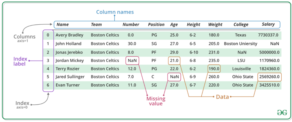 A labeled DataFrame with rows (observations) and columns (features). (Image: Lucasadvent, CC BY-SA 4.0, via Wikimedia Commons)
2.2 Reading and Writing Data
# Read CSV
df = pd.read_csv("employees.csv")

# Write to Excel
df.to_excel("output.xlsx", index=False)
2.3 Selecting Data
# Select column
print(df["Name"])

# Select multiple columns
print(df[["Name", "Salary"]])

# Select rows by condition
print(df[df["Age"] > 25])
Trace Table: Filtering Rows
| Step | Code | Result |
|---|---|---|
| 1 | df["Age"] > 25 |
Boolean mask: [False, True, True] |
| 2 | df[mask] |
Returns rows where Age > 25 |
2.4 Handling Missing Data
df = pd.DataFrame({
    "A": [1, 2, np.nan],
    "B": [np.nan, 2, 3],
    "C": [1, 2, 3]
})

# Drop rows with NaN
df_cleaned = df.dropna()

# Fill NaN with 0
df_filled = df.fillna(0)
Visual: Missing Data Handling
2.5 Grouping and Aggregation
```figure
{"type":"bar","labels":["Department A","Department B","Department C"],"values":[120000,180000,90000],"ylabel":"Total Salary (NPR)","caption":"Aggregated salaries by department"}
Group by "Department" and calculate average salary
df.groupby("Department")["Salary"].mean() Example: NEPSE Stock Analysis Suppose we have a DataFrame of NEPSE stock prices with columns:
Date: Trading date,Open: Opening price,High: Highest price,Low: Lowest price,Close: Closing price,Volume: Shares traded.
Code:
# Group by year and calculate average closing price
df["Date"] = pd.to_datetime(df["Date"])
df["Year"] = df["Date"].dt.year
avg_close = df.groupby("Year")["Close"].mean()
print(avg_close)
Output:
Year
2020    1200.50
2021    1350.75
2022    1420.30
2.6 Merging DataFrames
Pandas supports SQL-like joins:
# Merge two DataFrames on "EmployeeID"
employees = pd.DataFrame({
    "EmployeeID": [1, 2, 3],
    "Name": ["Alice", "Bob", "Charlie"]
})

salaries = pd.DataFrame({
    "EmployeeID": [1, 2, 4],
    "Salary": [50000, 60000, 70000]
})

merged = pd.merge(employees, salaries, on="EmployeeID", how="left")
Visual: Merge Types
graph LR
    A["employees\nID: 1,2,3"] --> B["salaries\nID: 1,2,4"]
    B --> C["merge(how='inner')\nID: 1,2"]
    B --> D["merge(how='left')\nID: 1,2,3 (NaN for 3)"]
    B --> E["merge(how='right')\nID: 1,2,4 (NaN for 4)"]
2.7 Time-Series Data
# Convert column to DatetimeIndex
df["Date"] = pd.to_datetime(df["Date"])
df.set_index("Date", inplace=True)

# Resample to monthly average
monthly_avg = df["Close"].resample("M").mean()
Real-World Example: Pathao’s Ride Demand Pathao uses Pandas to analyze ride demand trends by:
- Loading ride data (timestamp, pickup location, fare).
- Resampling by hour/day to find peak times.
- Grouping by location to optimize driver dispatch.
Code Snippet:
# Load ride data
rides = pd.read_csv("pathao_rides.csv")
rides["Timestamp"] = pd.to_datetime(rides["Timestamp"])
rides.set_index("Timestamp", inplace=True)

# Find hourly demand
hourly_demand = rides.resample("H").size()
print(hourly_demand.head())
Output:
Timestamp
2023-01-01 00:00:00    120
2023-01-01 01:00:00     80
2023-01-01 02:00:00     50
...
3. Visualization with Matplotlib
Pandas integrates with Matplotlib for plotting:
import matplotlib.pyplot as plt

# Line plot of stock prices
df["Close"].plot(title="NEPSE Closing Prices")
plt.show()

# Bar plot of sales by region
df.groupby("Region")["Sales"].sum().plot(kind="bar")
plt.show()
Visual: Stock Price Plot
4. NumPy vs. Pandas: Comparison
| Feature | NumPy | Pandas |
|---|---|---|
| Data Structure | Arrays (homogeneous) | DataFrames (heterogeneous) |
| Missing Data | No built-in support | NaN handling (dropna, fillna) |
| Operations | Vectorized math (e.g., arr + 5) |
Data manipulation (e.g., groupby) |
| Use Case | Numerical computing | Data analysis, cleaning, merging |
| Performance | Faster for math | Slower but feature-rich |
5. Real-World Applications
Example 1: eSewa Transaction Analysis
eSewa uses Pandas to:
- Detect fraud: Flag transactions with unusual amounts or frequencies.
- Customer segmentation: Group users by spending habits (e.g.,
groupby("CustomerID")["Amount"].sum()). - Visualize trends: Plot monthly transaction volumes.
Code:
# Load transactions
transactions = pd.read_csv("esewa_transactions.csv")
transactions["Date"] = pd.to_datetime(transactions["Date"])

# Monthly transaction volume
monthly_volume = transactions.resample("M", on="Date").size()
monthly_volume.plot(title="eSewa Monthly Transactions")
Example 2: Daraz Order Fulfillment
Daraz uses NumPy for:
- Inventory management: Calculate stock levels after bulk orders.
- Shipping cost estimation: Multiply weights (NumPy array) by rates.
Code:
# Calculate total shipping cost
weights = np.array([0.5, 1.2, 0.8])  # kg
rates = np.array([100, 150, 200])    # Rs/kg
costs = weights * rates
print(costs)  # [50, 180, 160]
Example 3: NTC Network Traffic Analysis
NTC monitors internet traffic using Pandas to:
- Detect anomalies: Identify spikes in data usage.
- Bandwidth allocation: Group by ISP and calculate average usage.
Code:
# Load traffic data
traffic = pd.read_csv("ntc_traffic.csv")
traffic["Timestamp"] = pd.to_datetime(traffic["Timestamp"])

# Hourly traffic by ISP
hourly_traffic = traffic.groupby([traffic["Timestamp"].dt.hour, "ISP"])["Usage"].sum()
print(hourly_traffic.head())
Exam Tip
NumPy:
- Remember broadcasting rules (compare shapes from the right).
- Practice array slicing and ufuncs (e.g.,
np.sqrt,np.sum). - Know how to reshape arrays (
np.reshape) and stack them (np.vstack,np.hstack).
Pandas:
- DataFrame creation: From dictionaries, lists, or CSV files.
- Filtering: Use boolean indexing (
df[df["Age"] > 30]). - Grouping:
groupby()+ aggregation (mean(),sum()). - Merging:
pd.merge()withhow="inner",how="left". - Time-series: Convert to
DatetimeIndexand useresample().
Common Pitfalls:
- Forgetting to convert strings to
datetime(pd.to_datetime). - Mixing up
merge()vs.concat()(usemergefor SQL-like joins). - Broadcasting errors (e.g., adding a 1D array to a 2D array without alignment).
- Forgetting to convert strings to
Exam Questions:
- Short answer: Define
DataFrame,Series, orbroadcasting. - Code: Write a function to:
- Filter a DataFrame by condition.
- Calculate statistics (mean, median) using NumPy.
- Merge two DataFrames.
- Problem-solving: Given a dataset (e.g., sales data), write code to:
- Clean missing values.
- Group and aggregate.
- Plot trends.
- Short answer: Define
Final Note: Master NumPy for math and Pandas for data. Always inspect your data (df.head(), df.info()) before analysis!
Based on the TU BITM syllabus for Programming with Python (IT243), unit 9.
Discussion
Loading…