Capital Structure & Leverage: Optimal Mix, Trade-offs & Real-World Impact

Core Concepts

What is Capital Structure?

Capital structure refers to the mix of debt and equity used by a company to finance its operations and growth. It answers:

• How much should a firm borrow (debt)?
• How much should it raise from shareholders (equity)?
• What is the optimal (best) balance?

Why does it matter? A company’s capital structure directly impacts:

• Cost of capital (cheaper debt vs. expensive equity).
• Risk (debt increases financial risk).
• Shareholder value (optimal structure maximizes firm value).

Theories Explaining Capital Structure

1. Modigliani-Miller (MM) Propositions (No-Tax World)

The foundational theory by Franco Modigliani and Merton Miller (1958, 1961) states:

• Proposition I: The value of a firm is independent of its capital structure (in a perfect world with no taxes, no transaction costs, and symmetric information).
  • Implication: Debt doesn’t change the total value of the firm.
• Proposition II: The cost of equity increases with leverage because equity becomes riskier as debt rises.
  • Formula: $$R_e=R_0+(R_0-R_d)\cdot \frac{D}{E}$$ Where:
    • $R_e$ = Cost of equity with leverage
    • $R_0$ = Cost of equity without leverage
    • $R_d$ = Cost of debt
    • $D/E$ = Debt-to-equity ratio

Visual: MM Proposition II in Action

Caption: As debt increases, the cost of equity rises linearly (assuming constant $R_0$ and $R_d$).

2. MM with Corporate Taxes (1963)

When taxes are introduced:

• Interest on debt is tax-deductible, while dividends are not.
• Value of the firm increases with debt because tax shields reduce the cost of capital.
  • Formula for firm value with taxes: $$V_L=V_U+T_c\cdot D$$ Where:
    • $V_L$ = Value of levered firm
    • $V_U$ = Value of unlevered firm
    • $T_c$ = Corporate tax rate
    • $D$ = Market value of debt

Real-World Tie-In:

• Nepal’s banks (e.g., NMB Bank, Global IME) use high debt-to-equity ratios because interest expenses reduce taxable income, boosting net profits.

3. Trade-Off Theory

In the real world, firms face:

• Tax benefits of debt (as per MM with taxes).
• Costs of financial distress (bankruptcy risk, agency costs).
• Optimal capital structure is where tax benefits ≈ distress costs.

Key Trade-Offs:

Visual: Trade-Off Theory Graph

![trade-off theory capital structure](/media/9d34caeec8e2b513d449.png "Optimal debt level where benefits = costs (Image: Suicup, CC BY-SA 3.0, via Wikimedia Commons)")

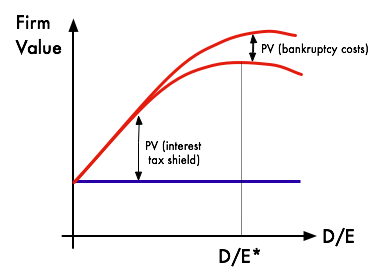
Caption: Firms choose debt levels where tax benefits outweigh distress costs (e.g., a Kathmandu retail chain may target 40% debt).

Types of Leverage

1. Operating Leverage

• Measures fixed vs. variable costs in operations.
• High operating leverage: High fixed costs (e.g., manufacturing plants).
  • Example: A Daraz warehouse has high fixed costs (rent, salaries) but low variable costs (per-unit shipping).
• Formula: $$\text{DOL}=\frac{\%\text{ Change in EBIT}}{\%\text{ Change in Sales}}$$
  • If DOL > 1, small sales changes lead to large EBIT changes (risky but profitable if sales grow).

Worked Example: Kathmandu Retail Shop Assume a shop has:

• Fixed costs (rent, salaries): NPR 500,000/month
• Variable costs (per unit): NPR 200
• Selling price: NPR 500
• Current sales: 5,000 units

Calculations:

1. EBIT = (Sales × (Price – Variable Cost)) – Fixed Costs = (5,000 × (500 – 200)) – 500,000 = NPR 1,500,000
2. DOL if sales rise by 10% (new sales = 5,500 units):
   • New EBIT = (5,500 × 300) – 500,000 = NPR 1,150,000
   • % Change in EBIT = (1,150,000 – 1,500,000)/1,500,000 = -23.3%
   • DOL = -23.3% / 10% = -2.33 (Absolute value shows high sensitivity).

Interpretation: A 10% drop in sales would wipe out EBIT. The shop should hedge risks (e.g., diversify products).

2. Financial Leverage

• Measures debt vs. equity in capital structure.
• High financial leverage: More debt → higher risk but potential for higher returns.
• Formula: $$\text{DFL}=\frac{\%\text{ Change in EPS}}{\%\text{ Change in EBIT}}$$
  • If DFL > 1, small EBIT changes lead to large EPS changes.

Worked Example: Ncell’s Capital Structure Assume Ncell has:

• EBIT: NPR 10 billion
• Interest: NPR 2 billion (10% debt)
• Tax rate: 25%
• Shares: 1 billion outstanding

Calculations:

1. EPS without debt:
   • Net Income = EBIT × (1 – Tax) = 10 × 0.75 = NPR 7.5 billion
   • EPS = 7.5 / 1 = NPR 7.5 per share
2. EPS with debt (10% of capital):
   • Net Income = (10 – 2) × 0.75 = NPR 6 billion
   • EPS = 6 / 1 = NPR 6 per share
   • Wait, this seems counterintuitive!

Correction: Financial leverage amplifies both gains and losses.

• If EBIT rises to NPR 12 billion:
  • Net Income = (12 – 2) × 0.75 = NPR 7.5 billion
  • EPS = 7.5 / 1 = NPR 7.5 (same as before, but riskier).
• If EBIT drops to NPR 8 billion:
  • Net Income = (8 – 2) × 0.75 = NPR 4.5 billion
  • EPS = 4.5 / 1 = NPR 4.5 (vs. NPR 6 without debt).

Key Insight: Debt magnifies volatility. Ncell must balance leverage to avoid financial distress.

3. Combined Leverage (Total Leverage)

• Measures how sensitive EPS is to sales changes.
• Formula: $$\text{DCL}=\text{DOL}\times \text{DFL}$$
• Example: If DOL = 1.5 and DFL = 2, then DCL = 3.
  • A 1% sales change → 3% EPS change.

Real-World Applications in Nepal

1. eSewa’s Capital Structure

• Debt: eSewa uses short-term debt (e.g., working capital loans) for liquidity.
• Equity: Backed by Nepal Investment Bank (major shareholder).
• Why?
  • High operating leverage (fixed tech infrastructure costs).
  • Low financial leverage to avoid bankruptcy risk (government-owned).

2. Pathao’s Leverage Strategy

• High debt: Pathao borrowed heavily for vehicle fleet expansion.
• Risk: If fuel prices rise or demand drops, high fixed costs (salaries, loan repayments) threaten profitability.
• Outcome: Pathao’s EPS is highly sensitive to sales changes (high DCL).

3. Nepal’s Banks (NMB, Global IME)

• Debt-to-Equity Ratio: ~60-70% (higher than global averages).
• Why?
  • Tax shield: Interest is deductible (25% corporate tax).
  • Regulatory limits: RBI Nepal caps debt at 80% of capital.
• Trade-Off: Higher debt increases risk of financial distress (e.g., 2015 NPL crisis).

The Accounting Cycle of Capital Structure Decisions

Key Steps:

1. Assess needs: Growth, expansion, or working capital?
2. Risk tolerance: Can the firm handle debt servicing?
3. Cost comparison: Debt is cheaper than equity (usually).
4. WACC: Weighted Average Cost of Capital guides the mix.
5. Optimal ratio: Where tax benefits > distress costs.
6. Monitor: Adjust if market conditions change (e.g., rising interest rates).

Numerical Example: Optimal Capital Structure for a Nepali Manufacturing Firm

Company: Everest Textiles Ltd. (produces fabrics for Daraz sellers). Current Data:

• EBIT: NPR 50 million
• Tax rate: 25%
• Current capital structure: 40% debt, 60% equity.
• Cost of debt ($R_d$): 10%
• Cost of equity ($R_e$) without leverage: 15%
• Market value of debt ($D$): NPR 40 million
• Market value of equity ($E$): NPR 60 million

Step 1: Calculate Unlevered Firm Value ($V_U$) $$V_U=E+D=60+40=\text{NPR 100 million}$$

Step 2: Calculate Cost of Equity with Leverage ($R_e$) Using MM Proposition II: $$R_e=R_0+(R_0-R_d)\cdot \frac{D}{E}=15+(15-10)\cdot \frac{40}{60}=16.67\%$$

Step 3: Calculate WACC $$\text{WACC}=\left(\frac{E}{V}\right)\cdot R_e+\left(\frac{D}{V}\right)\cdot R_d\cdot (1-T_c)$$ $$=\left(\frac{60}{100}\right)\cdot 16.67+\left(\frac{40}{100}\right)\cdot 10\cdot 0.75=10\%+3\%=13\%$$

Step 4: Tax Shield Benefit $$\text{Tax Shield}=D\cdot R_d\cdot T_c=40\times 10\%\times 25\%=\text{NPR 1 million}$$ Levered Value ($V_L$): $$V_L=V_U+\text{Tax Shield}=100+1=\text{NPR 101 million}$$

Step 5: Optimal Debt Adjustment Suppose Everest Textiles considers increasing debt to 60%:

• New $D=60$ million, $E=40$ million.
• New $R_e$: $$R_e=15+(15-10)\cdot \frac{60}{40}=22.5\%$$
• New WACC: $$\text{WACC}=0.4\times 22.5+0.6\times 10\times 0.75=9\%+4.5\%=13.5\%$$
• Distress Costs: Higher debt increases bankruptcy risk. If EBIT drops below NPR 30 million, interest payments (NPR 6 million) may exceed EBIT.

Conclusion: Everest Textiles should stick to 40% debt unless it can generate higher EBIT to justify the risk.

Advantages and Disadvantages of Leverage

Exam Tip

1. Memorize MM Propositions: Know the formulas and assumptions (no taxes vs. with taxes).
2. Calculate WACC: Always show steps for debt, equity, and tax adjustments.
3. Compare Theories: Trade-off vs. pecking order vs. signaling theories—know when each applies.
4. Real-World Examples: Link concepts to Nepali firms (e.g., banks’ high debt for tax shields, Pathao’s risky leverage).
5. Leverage Formulas:
   • DOL, DFL, DCL: Know how to compute and interpret.
   • Optimal capital structure: Balance tax benefits vs. distress costs.
6. Numerical Problems: Practice calculating EPS, WACC, and firm value under different leverage scenarios.

Common Pitfalls:

• Ignoring taxes in MM calculations.
• Assuming all debt is good (forget distress costs).
• Mixing operating and financial leverage in answers.

classDiagram
    class CapitalStructure {
        +mixOfDebtAndEquity
        +affectsFirmValue
        +tradesOffRiskAndReturn
    }
    class Leverage {
        +operatingLeverage
        +financialLeverage
        +combinedLeverage
    }
    class Theories {
        +MMNoTax
        +MMWithTax
        +TradeOff
        +PeckingOrder
    }
    CapitalStructure --> Leverage : "uses"
    CapitalStructure --> Theories : "explainedBy"
    Leverage --> "DOL" : "measures"
    Leverage --> "DFL" : "measures"
    Leverage --> "DCL" : "measures"