Curve & Surface Representation: Parametric, Bezier, B-Spline, Polygons & Fractals

Core Concepts

1. Parametric Curves

Parametric curves define shapes using a parameter $t$ (often $0\le t\le 1$) to map to coordinates $(x(t),y(t))$. They are fundamental for smooth, scalable graphics.

Key Properties

• Continuity: $G^0$ (connected), $G^1$ (tangent continuity), $G^2$ (curvature continuity).
• Degree: Number of control points minus one (e.g., cubic Bezier has degree 3).
• Convex Hull Property: The curve lies within the convex hull of its control points.

Example: Linear Interpolation

For points $P_0(x_0,y_0)$ and $P_1(x_1,y_1)$, the parametric form is: $$x(t)=x_0+t(x_1-x_0),y(t)=y_0+t(y_1-y_0),0\le t\le 1$$

2. Bezier Curves

Bezier curves are piecewise parametric curves defined by control points $P_0,P_1,\dots ,P_n$. They are widely used in CAD/CAM (e.g., Adobe Illustrator, AutoCAD).

Mathematical Definition

For $n$ control points, the Bezier curve $B(t)$ is: $$B(t)=\sum _{i=0}^n\left(\genfrac{}{}{0ex}{}{n}{i}\right)(1-t{)}^{n-i}{t}^i{P}_i,0\le t\le 1$$

• Bernstein Polynomials: $\left(\genfrac{}{}{0ex}{}{n}{i}\right)(1-t{)}^{n-i}{t}^i$ ensure smooth interpolation.
• De Casteljau’s Algorithm: A recursive method to compute points on the curve (useful for rendering).

Worked Example: Cubic Bezier Curve

Given control points $P_0(0,0)$, $P_1(1,2)$, $P_2(3,3)$, $P_3(4,0)$, compute $B(0.5)$:

1. Step 1: Compute intermediate points: $$Q_0=(1-t)P_0+t{P}_1=0.5P_0+0.5P_1=(0.5,1)$$ $$Q_1=0.5P_1+0.5P_2=(2,2.5)$$ $$Q_2=0.5P_2+0.5P_3=(3.5,1.5)$$
2. Step 2: Compute next level: $$R_0=0.5Q_0+0.5Q_1=(1.25,1.75)$$ $$R_1=0.5Q_1+0.5Q_2=(2.75,2)$$
3. Step 3: Final point: $$B(0.5)=0.5R_0+0.5R_1=(2,1.875)$$

Plot Sketch:

P0(0,0) ---- P1(1,2)
           /    \
          /      \
P2(3,3) ---- P3(4,0)

The curve starts at $P_0$, ends at $P_3$, and is "pulled" toward $P_1$ and $P_2$.

Advantages/Disadvantages

3. B-Spline Curves

B-splines (Basis Splines) generalize Bezier curves with:

• Knot vectors: Define parameter ranges for segments.
• Local control: Adjusting one control point affects only a subset of the curve.
• Degree $p$: Typically cubic ($p=3$) for smoothness.

Mathematical Definition

For a knot vector $U=\{u_0,u_1,\dots ,u_{m+p}\}$ and control points $P_i$, the B-spline curve is: $$C(t)=\sum _{i=0}^n{N}_{i,p}(t)P_i,t\in [u_p,u_m]$$ where $N_{i,p}(t)$ are B-spline basis functions.

Comparison: Bezier vs. B-Spline

Worked Example: Quadratic B-Spline

Given control points $P_0(0,0)$, $P_1(1,2)$, $P_2(2,0)$ and knot vector $U=\{0,0,0,1,2,2,2\}$, compute $C(1)$:

• Basis functions $N_{0,2}(1)=0.5$, $N_{1,2}(1)=1$, $N_{2,2}(1)=0.5$.
• $C(1)=0.5P_0+1P_1+0.5P_2=(1,2)$.

4. Surface Representation

A. Polygon Meshes

• Polygon Table: Stores vertices, edges, and faces (e.g., triangles, quadrilaterals).
  • Vertex List: $(x,y,z)$ coordinates.
  • Face List: Indices referencing vertices (e.g., Face 1: 0,1,2 for vertices $P_0,P_1,P_2$).
• Applications: 3D modeling (e.g., Blender, Maya), game engines.

B. Parametric Surfaces

Extend curves to 2D using two parameters $u$ and $v$: $$S(u,v)=\sum _{i=0}^m\sum _{j=0}^n{B}_{i,p}(u)B_{j,q}(v)P_{i,j}$$

• Bezier Surface: Tensor product of Bezier curves.
• B-Spline Surface: Tensor product of B-splines.

C. Fractals

• Definition: Self-similar structures generated iteratively (e.g., Mandelbrot set, Koch snowflake).
• Properties:
  • Recursion: Simple rules applied repeatedly.
  • Infinite Detail: Zooming reveals new patterns.
• Applications: Procedural generation, terrain modeling, artistic designs.

Mermaid Diagram: Fractal Construction

flowchart TD
    A["Start with\nInitial Shape"] --> B["Apply\nTransformation"]
    B --> C["Check\nTermination?"]
    C -->|No| D["Add to\nComposite"]
    D --> B
    C -->|Yes| E["Render\nFractal"]

5. Curve and Surface Interpolation

• Interpolation: Curve passes through all control points (e.g., Lagrange polynomials).
• Approximation: Curve fits control points but doesn’t pass through them (e.g., least-squares fitting).
• Example: Catmull-Rom splines (interpolating B-splines).

Exam Tip

1. Bezier Curves:

   • Memorize the De Casteljau algorithm for computation.
   • Plot rough sketches for control points (e.g., "humps" for $P_1$ and $P_{n-1}$).
   • Common Pitfall: Forgetting the curve only passes through $P_0$ and $P_n$.

2. B-Splines:

   • Compare with Bezier curves in terms of local control and knot vectors.
   • Know the degree affects smoothness (higher degree = smoother but computationally expensive).

3. Surface Representation:

   • Explain polygon meshes using vertex/face tables.
   • For fractals, describe self-similarity and recursive generation.

4. Numerical Questions:

   • Always show step-by-step calculations (e.g., De Casteljau).
   • For $u=0.5$, compute intermediate points explicitly.

5. Diagrams:

   • Draw control polygons for Bezier/B-spline curves.
   • Label axes and key points (e.g., $P_0,P_n$, curve direction).

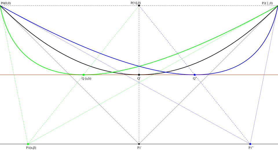Example of a cubic Bezier curve with 4 control points (Image: 丁志仁, CC BY-SA 4.0, via Wikimedia Commons)