Computer GraphicsUnit 113 min read
Computer Graphics Basics: Definitions, Systems, & Rendering Pipeline
Unit 1 of Computer Graphics introduces core concepts like raster vs. vector graphics, the rendering pipeline, human perception, and machine-independent standards (e.g., OpenGL). It explains how 3D scenes are transformed into 2D images, the role of shading models, and the significance of graphics standards in applicatio
1. Introduction to Computer Graphics
Computer Graphics (CG) is the study of generating visual content using computers, combining principles from mathematics, physics, and computer science. It enables the creation of 2D/3D images, animations, simulations, and virtual environments for applications like gaming, film, medical imaging, and CAD.
1.1 Definition and Scope
- Computer Graphics: The art and science of creating static/dynamic visual content using computational techniques.
- Applications:
- Entertainment: Movies (Toy Story), games (Call of Duty), animations.
- Medical: 3D organ modeling, surgical simulations.
- Engineering: CAD/CAM (e.g., AutoCAD), architectural visualization.
- Scientific Visualization: Weather forecasting, molecular modeling.
1.2 Human Perception and Realism
- Human Vision System:
- Eyes detect light reflected off objects (wavelengths: ~400–700 nm).
- Brain interprets color, depth, motion, and shading via cues like:
- Perspective: Parallel lines converge at a vanishing point.
- Texture: Surface details (e.g., wood grain).
- Shadows/Lighting: Simulates real-world illumination.
- Realism in CG:
- Achieved through physically based rendering (PBR), accurate lighting models (e.g., Phong, Blinn-Phong), and ray tracing.
- Challenge: Balancing computational cost vs. visual fidelity.
2. Graphics Systems: Raster vs. Vector
Graphics systems are classified into two primary paradigms:
2.1 Raster Graphics (Bitmap)
- Definition: Images represented as a grid of pixels (picture elements), each with a color value.
- How it works:
- Each pixel stores RGB (or RGBA) values (e.g., 24-bit color: 8 bits per channel).
- Resolution-dependent: Scaling causes pixelation.
- Advantages:
- Photorealistic images (e.g., photos, textures).
- Simple to render with hardware acceleration (GPUs).
- Disadvantages:
- Large file sizes for high-resolution images.
- No inherent scaling (loss of quality).
- Examples: JPEG, PNG, BMP.
- Applications: Digital photography, web images, video frames.
2.2 Vector Graphics
- Definition: Images defined by mathematical equations (e.g., lines, curves, polygons) using paths and anchors.
- How it works:
- Scalable without quality loss (resolution-independent).
- Uses primitives: Points, lines, Bézier curves, polygons.
- Advantages:
- Small file sizes, infinite scalability.
- Editable (e.g., Adobe Illustrator).
- Disadvantages:
- Complex for photorealistic images.
- Slower rendering for complex scenes.
- Examples: SVG, PDF, AI (Adobe Illustrator).
- Applications: Logos, icons, typography, technical drawings.
Comparison Table
| Feature | Raster Graphics | Vector Graphics |
|---|---|---|
| Representation | Pixel grid | Mathematical paths |
| Scalability | Lossy (pixelation) | Lossless |
| File Size | Large (high-res) | Small |
| Editing | Difficult (pixel-level) | Easy (path manipulation) |
| Hardware Support | GPU-optimized | CPU-intensive |
| Use Case | Photos, textures | Logos, illustrations |
3. The Rendering Pipeline
The 3D viewing pipeline transforms a 3D world into a 2D image on screen. Key stages:
flowchart TD
    A[3D World Coordinates] --> B[Modeling Transform]
    B --> C[Viewing Transform]
    C --> D[Projection Transform]
    D --> E[Viewport Transform]
    E --> F[Rasterization]
    F --> G[2D Screen Image]
3.1 Steps in the Pipeline
- Modeling Transform:
- Objects defined in world coordinates (e.g., a cube at
(1, 2, 3)). - Transformed via translation, rotation, scaling (using matrices).
- Objects defined in world coordinates (e.g., a cube at
- Viewing Transform:
- Converts world coordinates to eye (camera) coordinates.
- Defines viewpoint, up-vector, and look-at direction.
- Projection Transform:
- Converts 3D to 2D using perspective or orthographic projection.
- Perspective: Simulates depth (vanishing point).
- Orthographic: Parallel projection (no depth distortion).
- Viewport Transform:
- Maps 2D coordinates to screen pixels (e.g., 1920×1080).
- Rasterization:
- Converts primitives (lines, polygons) into pixels (scan conversion).
- Shading and Texturing:
- Applies lighting models (e.g., Phong shading) and textures.
3.2 Example: 2D Rotation
Definition: Rotating a point (x, y) by angle θ about the origin.
Rotation Matrix:
Worked Example:
Rotate (2, 3) by 45° (θ = 45°, cosθ = sinθ = √2/2 ≈ 0.707).
New Coordinates: (-0.707, 3.535).
4. Rendering and Image Synthesis
4.1 Rendering
- Definition: The process of generating a 2D image from a 3D model by simulating light interaction.
- Key Techniques:
- Scanline Rendering: Renders polygons line-by-line.
- Ray Tracing: Simulates light rays (realistic shadows/reflections).
- Rasterization: Converts geometry to pixels (used in real-time graphics).
4.2 Image Synthesis vs. Rendering
| Rendering | Image Synthesis |
|---|---|
| Focuses on real-time or offline image generation. | Focuses on procedural generation (e.g., fractals, textures). |
| Uses lighting models (Phong, Blinn-Phong). | Uses algorithmic patterns (e.g., Perlin noise). |
| Output: Photorealistic images. | Output: Abstract/artistic images. |
| Example: Movie frames. | Example: Generative art (e.g., DALL·E). |
4.3 Polygon Rendering Methods
- Wireframe Rendering:
- Displays only edges of polygons (fast but unrealistic).
- Flat Shading:
- Assigns a single color per polygon (no smooth gradients).
- Gouraud Shading:
- Interpolates vertex colors across a polygon (smoother than flat shading).
- Phong Shading:
- Interpolates surface normals, then computes lighting per pixel (high quality).
Phong Shading Formula:
- : Final intensity.
- : Ambient/diffuse/specular coefficients.
- : Light direction.
- : Surface normal.
- : Reflection vector.
- : View direction.
Advantages:
- Smooth gradients, realistic highlights. Disadvantages:
- Computationally expensive (per-pixel calculations).
5. Machine-Independent Graphics Standards
5.1 Need for Standards
- Problem: Graphics hardware/software varies (e.g., Windows vs. Linux, NVIDIA vs. AMD GPUs).
- Solution: APIs (Application Programming Interfaces) provide a consistent interface for developers.
- Benefits:
- Portability: Code runs across platforms.
- Abstraction: Hides hardware details.
- Performance: Optimized libraries (e.g., GPU acceleration).
5.2 Key Standards
| Standard | Description | Example Libraries |
|---|---|---|
| OpenGL | Cross-platform API for 2D/3D rendering. | GLUT, GLFW |
| DirectX | Microsoft’s API for Windows gaming/graphics. | Direct3D, Direct2D |
| WebGL | JavaScript API for browser-based 3D graphics. | Three.js, Babylon.js |
| Vulkan | Low-level API for high-performance graphics (successor to OpenGL). | MoltenVK (macOS) |
| SVG | Vector graphics standard for web. | Inkscape, Adobe Illustrator |
5.3 How Standards Work
classDiagram
    class Developer {
        +Writes code using OpenGL
    }
    class OpenGL {
        +Provides functions like glVertex(), glDraw()
    }
    class GPU {
        +Renders polygons
    }
    class Monitor {
        +Displays pixels
    }
    Developer --> OpenGL : Uses
    OpenGL --> GPU : Calls
    GPU --> Monitor : Renders
6. Filling Algorithms
Used to fill polygons with color/texture. Two primary methods:
6.1 Boundary Fill Algorithm
- How it works:
- Start at a seed point inside the polygon.
- Check if the point is inside the boundary.
- Fill the point, then recursively fill adjacent points (4-connected or 8-connected).
- Pseudocode:
def boundary_fill(x, y, fill_color): if (x, y) is outside boundary: return if (x, y) is already filled: return set_pixel(x, y, fill_color) boundary_fill(x+1, y, fill_color) # 4-connected boundary_fill(x-1, y, fill_color) boundary_fill(x, y+1, fill_color) boundary_fill(x, y-1, fill_color) - Advantages: Simple, works for any shape.
- Disadvantages: Slow for complex polygons (recursion overhead).
6.2 Flood Fill Algorithm
- How it works:
- Similar to boundary fill but does not check boundaries.
- Fills all connected pixels of a given color (e.g., paint bucket tool).
- Use Case: Image editing (e.g., changing background color).
Comparison
| Feature | Boundary Fill | Flood Fill |
|---|---|---|
| Boundary Check | Yes (uses polygon edges) | No (fills connected pixels) |
| Speed | Slower (recursive) | Faster (iterative) |
| Use Case | Polygon filling in CG | Image editing |
7. Shadows and Lighting Models
7.1 Shadow Detection
- Methods:
- Shadow Mapping:
- Render scene from light’s perspective to create a depth map.
- Compare depth values to detect shadows.
- Ray Casting:
- Trace rays from light to object; blockage = shadow.
- Shadow Volumes:
- Extend polygons into 3D to form "volumes"; clip against view frustum.
- Shadow Mapping:
- Challenges:
- Aliasing: Jagged edges in shadows.
- Performance: Real-time shadow mapping requires GPU optimization.
- Soft Shadows: Requires complex algorithms (e.g., Percentage-Closer Filtering).
7.2 Lighting Models
- Ambient Lighting:
- Uniform light everywhere (no direction).
- Diffuse Lighting:
- Light scatters equally in all directions (Lambertian reflection).
- Specular Lighting:
- Highlights (mirror-like reflections).
- Phong Reflection Model:
- Combines ambient, diffuse, and specular components (as shown earlier).
8. Exam Tip
Key Focus Areas for TU Exams
- Definitions:
- Differentiate raster vs. vector, rendering vs. image synthesis, boundary vs. flood fill.
- Know the 3D viewing pipeline stages (modeling → projection → viewport).
- Mathematical Derivations:
- Rotation matrix (2D/3D), translation/scaling matrices.
- Phong shading formula (derive intensity components).
- Algorithms:
- Boundary fill pseudocode (trace execution for a simple polygon).
- Line drawing algorithms (e.g., DDA, Bresenham’s) may appear in later units but are foundational.
- Applications:
- Explain where vector graphics (logos) vs. raster graphics (photos) are used.
- Describe real-world uses of OpenGL/DirectX (e.g., gaming, VR).
- Diagrams:
- Draw the 3D viewing pipeline or Phong reflection model components.
- Common Pitfalls:
- Confusing rasterization vs. ray tracing: Rasterization is for polygons; ray tracing simulates light rays.
- Forgetting to normalize vectors in lighting calculations.
- Mixing up Gouraud vs. Phong shading: Gouraud interpolates colors; Phong interpolates normals.
Sample Exam Questions and Answers
| Question | Key Points to Include |
|---|---|
| "Define 2D rotation and derive the rotation matrix." | Matrix: . Show derivation from trigonometry. |
| "Differentiate between raster and vector graphics." | Table comparison (resolution, scalability, use cases). |
| "Explain the 3D viewing pipeline." | 5-step flow (modeling → projection → viewport → rasterization). Include Mermaid diagram. |
| "What is Phong shading? Mention advantages/disadvantages." | Per-pixel normal interpolation; advantage: smooth highlights; disadvantage: computationally heavy. |
| "Why are machine-independent standards needed?" | Portability, abstraction, performance (e.g., OpenGL works on any GPU). |
Mark Distribution Tips
- Definitions (2–3 marks): Be precise (e.g., "Raster graphics use pixels; vector uses paths").
- Derivations (4–5 marks): Show steps (e.g., rotation matrix derivation).
- Diagrams (3 marks): Neat, labeled flowcharts (e.g., pipeline stages).
- Applications (2 marks): Give 1–2 real-world examples (e.g., "OpenGL is used in Unity games").
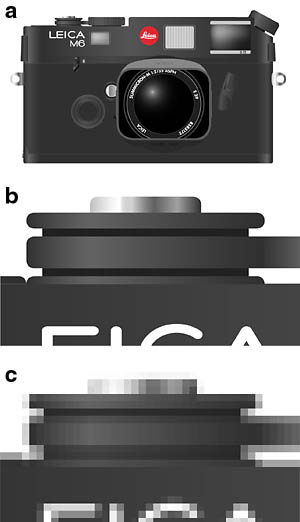 Side-by-side comparison of a pixelated image (raster) and a scalable logo (vector). (Image: User Agateller on en.wikipedia, CC BY-SA 3.0, via Wikimedia Commons)
Based on the TU BSc CSIT syllabus for Computer Graphics (CSC214), unit 1.
Discussion
Loading…