Computer GraphicsUnit 210 min read
Line Drawing Algorithms: DDA, Bresenham, Cohen-Sutherland
Unit 2 of Computer Graphics covers fundamental line-drawing algorithms (DDA, Bresenham), line-clipping (Cohen-Sutherland), and their mathematical foundations, including error analysis, region codes, and optimization trade-offs. Students learn to derive algorithms, trace pixel paths, and apply them to real-world scenari
Core Concepts
1. Why Line Drawing Matters
Lines are the primitive building blocks of computer graphics. Efficient algorithms determine:
- Speed: Real-time rendering (e.g., games, simulations).
- Quality: Anti-aliasing, smooth curves.
- Precision: Avoiding jagged edges (staircase effect).
Applications:
- CAD/CAM: Technical drawings.
- Animation: Skeletal rigging, motion paths.
- User Interfaces: Icons, buttons, graphs.
2. Digital Line Representation
A line between two points and is represented as a sequence of rasterized pixels (discrete points on a grid). The challenge is to:
- Approximate the continuous line with minimal error.
- Optimize computational cost (fewer calculations = faster rendering).
Key Definitions:
- Pixel: Smallest addressable screen element (e.g.,
(x, y)). - Staircase Effect: Jagged appearance due to discrete sampling.
- Error Term: Difference between the ideal line and the rasterized path.
3. Digital Differential Analyzer (DDA) Algorithm
The simplest incremental line-drawing algorithm, based on parametric equations.
How It Works
- Calculate slope .
- Incrementally plot pixels using:
- , where increases from 0 to 1.
- Round to the nearest integer (or vice versa if ).
Algorithm Steps
def DDA(x0, y0, x1, y1):
    dx = x1 - x0
    dy = y1 - y0
    steps = max(abs(dx), abs(dy))  # Number of increments

    x_inc = dx / steps
    y_inc = dy / steps

    x, y = x0, y0
    plot(x, y)  # Draw pixel

    for _ in range(steps):
        x += x_inc
        y += y_inc
        plot(round(x), round(y))
Example: Trace from (2, 3) to (10, 8)
| Step | Pixel Plotted | ||
|---|---|---|---|
| 0 | 2.0 | 3.0 | (2, 3) |
| 1 | 2.8 | 3.6 | (3, 4) |
| 2 | 3.6 | 4.2 | (4, 4) |
| ... | ... | ... | ... |
| 8 | 10.0 | 8.0 | (10, 8) |
Pros:
- Simple to implement.
- Works for any slope.
Cons:
- Floating-point operations (slow on early hardware).
- Rounding errors accumulate, causing visible gaps.
4. Bresenham’s Line Algorithm
Optimized for integer arithmetic, making it faster and more efficient than DDA.
Key Idea
- Error term () tracks deviation from the ideal line.
- Decision parameter () determines the next pixel:
- If , choose the pixel closer to the major axis (x or y).
- Else, adjust both axes.
Derivation
For a line with slope :
- Error equation: (Error accumulates as we move right.)
- Decision parameter:
- If , plot (steeper slope).
- Else, plot (shallower slope).
Algorithm Steps
def Bresenham(x0, y0, x1, y1):
    dx = abs(x1 - x0)
    dy = abs(y1 - y0)
    sx = 1 if x0 < x1 else -1
    sy = 1 if y0 < y1 else -1
    err = dx - dy

    while True:
        plot(x0, y0)
        if x0 == x1 and y0 == y1: break
        e2 = 2 * err
        if e2 > -dy:
            err -= dy
            x0 += sx
        if e2 < dx:
            err += dx
            y0 += sy
Example: Trace from (6, 12) to (10, 5)
| Step | Error | Decision | |
|---|---|---|---|
| 0 | (6, 12) | 0 | Start |
| 1 | (7, 12) | -7 | → move right |
| 2 | (8, 11) | -3 | → move right & down |
| 3 | (9, 11) | 1 | → move right |
| 4 | (10, 10) | 5 | → move right & down |
| 5 | (10, 5) | - | End |
Pros:
- Integer arithmetic (no floating-point errors).
- Faster than DDA (fewer operations).
- Smoother lines (better error correction).
Cons:
- Complex derivation (harder to understand intuitively).
- Limited to axis-aligned lines (extensions needed for arbitrary slopes).
5. Comparison: DDA vs. Bresenham
| Feature | DDA | Bresenham |
|---|---|---|
| Arithmetic | Floating-point | Integer-only |
| Speed | Slower (FPU operations) | Faster (integer ops) |
| Error Handling | Rounding errors | Error term correction |
| Implementation | Simple | Complex (derivation needed) |
| Use Case | Prototyping | Real-time rendering (games, UI) |
6. Line Clipping: Cohen-Sutherland Algorithm
Clips a line segment to a rectangular window using region codes and trivial rejection.
Key Concepts
- Window: The visible rectangle .
- Viewport: Where the clipped line is drawn (often the screen).
- Region Codes: 4-bit codes indicating a point’s position relative to the window.
0001: Left of window0010: Right of window0100: Below window1000: Above window
Algorithm Steps
- Compute region codes for both endpoints.
- Trivial Acceptance/Rejection:
- If both codes are
0000→ accept (fully inside). - If bitwise AND is non-zero → reject (fully outside).
- If both codes are
- Clip iteratively:
- Find the closest edge to the line.
- Compute intersection with that edge.
- Update the endpoint and its region code.
- Repeat until acceptance or rejection.
Example: Clip Line (10, 10) to (60, 30) in Window (15, 15) to (25, 25)
- Region Codes:
- :
1001(left + below) - :
0110(right + above)
- :
- Bitwise AND:
1001 & 0110 = 0000→ not trivial. - Closest Edge: Left edge ().
- Intersection: .
- New (rounded).
- Repeat:
- New codes: , .
- Next closest edge: Bottom ().
- Intersection: .
- New .
- Final Check:
- Both points inside → accept clipped line from (15, 12) to (22, 15).
Pros:
- Efficient (early rejection).
- Works for any rectangle.
Cons:
- Only rectangular windows.
- Complex for non-axis-aligned clipping (use Liang-Barsky for generalization).
7. Midpoint Circle Algorithm
Extends Bresenham’s idea to circles using symmetry.
Key Idea
- Symmetry: Only calculate 1/8th of the circle (rest mirrored).
- Decision Parameter: , where is the error function.
Algorithm Steps
def MidpointCircle(xc, yc, r):
    x = 0
    y = r
    p = 1 - r  # Initial decision parameter

    while x <= y:
        plot(xc + x, yc + y)  # Octant 1
        plot(xc - x, yc + y)  # Octant 2
        plot(xc + x, yc - y)  # Octant 8
        plot(xc - x, yc - y)  # Octant 7

        if p < 0:
            p += 2*x + 3
        else:
            p += 2*(x - y) + 5
            y -= 1
        x += 1
Example: Circle with Radius 5
| Points Plotted | |||
|---|---|---|---|
| 0 | 5 | 1 - 5 = -4 | (5,5), (5,-5), (-5,5), (-5,-5) |
| 1 | 5 | -4 + 2(0) + 3 = -1 | ... |
| 2 | 5 | -1 + 2(1) + 3 = 4 | ... |
| 2 | 4 | 4 + 2(2-4) + 5 = 3 | ... |
Pros:
- Efficient (only 1/8th calculated).
- Integer arithmetic.
Cons:
- Limited to circles (extensions for ellipses exist).
8. Applications and Extensions
Real-World Uses
- CAD Software: AutoCAD, SolidWorks (line clipping for views).
- Games: Wireframe rendering, minimaps.
- Medical Imaging: MRI/CT scan line tracing.
Advanced Topics
- Anti-Aliasing: Smooths jagged lines (e.g., supersampling).
- Parametric Curves: Bézier, B-splines (for smooth lines).
- 3D Line Drawing: Perspective projection, depth testing.
Exam Tip
What Examiners Look For
Derivations:
- Show step-by-step math for Bresenham/DDA (e.g., error term, decision parameter).
- Example: For Bresenham, derive .
Tracing Examples:
- Plot every pixel in the path (e.g., Bresenham from (2,3) to (10,8)).
- Label error terms in midpoint circle.
Region Codes:
- Binary masks for Cohen-Sutherland (e.g.,
1001for left + below). - Show intersection calculations with edges.
- Binary masks for Cohen-Sutherland (e.g.,
Comparisons:
- Table format for DDA vs. Bresenham (speed, error, use case).
- Pros/cons of clipping algorithms (e.g., Cohen-Sutherland vs. Liang-Barsky).
Common Pitfalls
- Floating-point rounding in DDA (use Bresenham for precision).
- Symmetry assumptions in circle algorithms (only plot 1/8th).
- Edge cases in clipping (e.g., vertical/horizontal lines).
Model Answer Structure
**Part A: Derive Bresenham’s Algorithm**
1. Start with line equation .
2. Define error term .
3. Show decision parameter .
4. **Trace example**: Plot (6,12) to (10,5) with table of , , and decisions.
**Part B: Cohen-Sutherland Clipping**
1. Define region codes for and .
2. Show bitwise AND → non-trivial.
3. **Clip iteratively**:
- Left edge intersection → new .
- Bottom edge intersection → new .
4. Final clipped line: to .
**Part C: Comparison**
| Algorithm | Advantage | Disadvantage |
|----------------|-------------------------|-----------------------|
| DDA | Simple | Floating-point errors |
| Bresenham | Integer arithmetic | Complex derivation |
| Cohen-Sutherland| Fast rejection | Only rectangles |
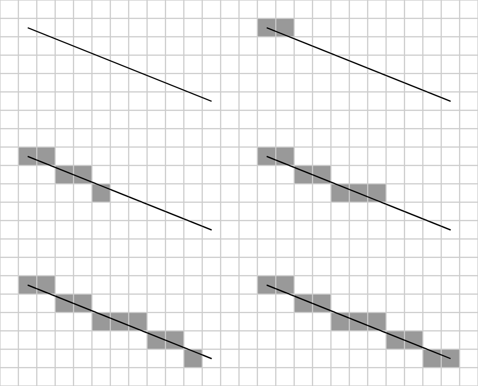 Example pixel path from (0,0) to (5,3) using Bresenham’s method (Image: Dnttllthmmnm, CC BY-SA 4.0, via Wikimedia Commons)
flowchart TD
    A[Start: Line Endpoints] --> B{Both Inside?}
    B -->|Yes| C[Accept Line]
    B -->|No| D{Bitwise AND Non-Zero?}
    D -->|Yes| E[Reject Line]
    D -->|No| F[Find Closest Edge]
    F --> G[Compute Intersection]
    G --> H[Update Endpoint]
    H --> B
Based on the TU BSc CSIT syllabus for Computer Graphics (CSC214), unit 2.
Discussion
Loading…