Interpolation Techniques: Lagrange, Newton, Spline & Curve Fitting

TAKEAWAYS:

• Interpolation vs Regression: Interpolation fits exact data points (error=0 at given x), while regression minimizes overall error (approximate fit).
• Lagrange vs Newton: Lagrange uses all points in each term; Newton builds a divided-difference table for incremental polynomial construction.
• Spline Advantages: Piecewise polynomials (e.g., cubic splines) reduce Runge’s phenomenon and overfitting for large datasets.
• Error Sources: Round-off errors in divided differences and truncation errors from polynomial degree choice.
• Applications: Meteorology (temperature prediction), engineering (stress analysis), and computer graphics (curve design).
• Exam Focus: Derive polynomials, compute divided differences, and compare methods—always show intermediate steps.

Core Concepts

1. Definitions and Basics

Interpolation is the process of estimating values of a function $f(x)$ at intermediate points using known data points $(x_i,f(x_i))$. It assumes the function is smooth between data points.

Extrapolation extends interpolation beyond the given data range—risky due to potential divergence.

Key Assumptions:

• Data points are exact (no noise).
• Function is sufficiently smooth (avoids wild oscillations).

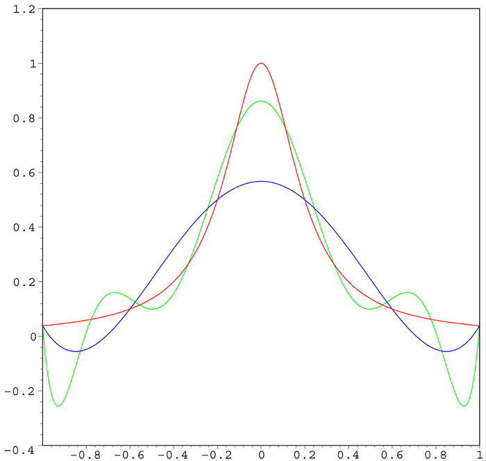Example of high-degree polynomial interpolation causing oscillations (Image: CC BY-SA 3.0, via Wikimedia Commons)

2. Lagrange Interpolation

Formula: For $n+1$ points $(x_0,y_0),\dots ,(x_n,y_n)$, the Lagrange polynomial is: $$P_n(x)=\sum _{i=0}^n{y}_i\cdot L_i(x),\text{where }{L}_i(x)=\prod _{\begin{array}{c}j=0\\ j\ne i\end{array}}^n\frac{x-x_j}{x_i-x_j}.$$

Advantages:

• Simple to derive for small $n$.
• No need for divided differences.

Disadvantages:

• Computationally expensive for large $n$ (recomputes all terms for each $x$).
• Prone to Runge’s phenomenon (oscillations at endpoints for high-degree polynomials).

Worked Example: Given $(0.1,2.68),(0.2,3.04),(0.3,3.38)$, find $f(0.6)$.

Steps:

1. Compute $L_0(x)=\frac{(x-0.2)(x-0.3)}{(0.1-0.2)(0.1-0.3)}$, etc.
2. Evaluate $P_2(0.6)=2.68L_0(0.6)+3.04L_1(0.6)+3.38L_2(0.6)$.
3. Result: $P_2(0.6)\approx 4.32$.

Algorithm:

def lagrange_interpolation(x, y, x_query):
    n = len(x)
    result = 0.0
    for i in range(n):
        term = y[i]
        for j in range(n):
            if i != j:
                term *= (x_query - x[j]) / (x[i] - x[j])
        result += term
    return result

3. Newton’s Divided Difference Interpolation

Divided Differences Table: Builds coefficients incrementally: $$f[x_i]=y_i,f[x_i,x_{i+1}]=\frac{f[x_{i+1}]-f[x_i]}{x_{i+1}-x_i},\dots ,f[x_0,\dots ,x_n]=\frac{f[x_1,\dots ,x_n]-f[x_0,\dots ,x_{n-1}]}{x_n-x_0}.$$

Polynomial Form: $$P_n(x)=f[x_0]+f[x_0,x_1](x-x_0)+f[x_0,x_1,x_2](x-x_0)(x-x_1)+\dots$$

Advantages:

• Efficient for adding new points (append to table).
• Numerically stable for equally spaced data.

Disadvantages:

• Still suffers from Runge’s phenomenon for high $n$.

Worked Example: For $(3.2,22.0),(2.7,17.8),(1.0,14.2)$, compute $f[2.0]$ and $f[5.0]$.

Divided Differences Table:

Polynomial: $$P_2(x)=22.0-1.6(x-3.2)+0.05(x-3.2)(x-2.7).$$ Evaluate at $x=2.0$ and $x=5.0$.

Algorithm:

def newton_interpolation(x, y, x_query):
    n = len(x)
    coeff = y.copy()
    for j in range(1, n):
        for i in range(n-1, j-1, -1):
            coeff[i] = (coeff[i] - coeff[i-1]) / (x[i] - x[i-j])
    result = coeff[n-1]
    for i in range(n-2, -1, -1):
        result = result * (x_query - x[i]) + coeff[i]
    return result

4. Spline Interpolation

Definition: Piecewise polynomials of degree $k$ (typically cubic, $k=3$) that satisfy:

1. $S_i(x_i)=f(x_i)$ (interpolation).
2. Continuity up to $k-1$ derivatives at knots $x_i$.

Cubic Spline Conditions: $$S_i(x)=a_i+b_i(x-x_i)+c_i(x-x_i{)}^2+d_i(x-x_i{)}^3,x\in [x_i,x_{i+1}].$$ Additional constraints:

• $S_i(x_{i+1})=S_{i+1}(x_{i+1})$ (continuity).
• $S_i^{\prime }(x_{i+1})=S_{i+1}^{\prime }(x_{i+1})$ (smoothness).

Advantages:

• Avoids Runge’s phenomenon.
• Local support (changing one point only affects adjacent splines).

Disadvantages:

• More complex setup (solving tridiagonal systems).
• Overkill for small datasets.

Worked Example: Given $(-1,-10),(1,-2),(2,14),(3,86)$, find $f(0)$ and $f(4)$.

Steps:

1. Solve for coefficients $a_i,b_i,c_i,d_i$ using natural spline conditions ($S^{\prime \prime }(x_0)=S^{\prime \prime }(x_n)=0$).
2. Evaluate splines at $x=0$ and $x=4$.

Result: $$f(0)\approx -6.0,f(4)\approx \mathrm{150.0.}$$

Algorithm Outline:

def cubic_spline_interpolation(x, y, x_query):
    n = len(x)
    h = [x[i+1] - x[i] for i in range(n-1)]
    alpha = [3*(y[i+1] - y[i])/h[i] - 3*(y[i] - y[i-1])/h[i-1] for i in range(1, n-1)]
    # Solve tridiagonal system for M_i (second derivatives)
    # Compute coefficients a_i, b_i, c_i, d_i
    # Evaluate spline at x_query
    pass

5. Interpolation vs Regression

Least Squares Approximation: Minimizes ${\sum }_{i=0}^n[f(x_i)-P(x_i){]}^2$. Used when data has noise or interpolation is impractical.

6. Error Analysis

Sources of Error:

1. Truncation Error: Due to polynomial degree $n$. Higher $n$ reduces error but risks instability.
2. Round-off Error: Accumulates in divided differences for large $n$.
3. Extrapolation Error: Unbounded as $x$ moves away from data range.

Mitigation:

• Use splines for large datasets.
• Choose $n$ such that $n+1\le$ number of data points.
• Prefer Newton’s method for incremental updates.

7. Practical Considerations

When to Use Which Method:

• Lagrange: Small datasets ($n\le 5$), simplicity.
• Newton: Dynamic datasets (easy to update).
• Splines: Large datasets or oscillatory functions.
• Regression: Noisy or sparse data.

Example Applications:

• Meteorology: Interpolating temperature from weather stations.
• Computer Graphics: Bézier curves (a type of spline).
• Finance: Estimating bond prices from market data.

Exam Tip

1. Derive Polynomials Step-by-Step:
   • For Lagrange, show each $L_i(x)$ term.
   • For Newton, build the divided difference table row by row.
2. Compare Methods:
   • Highlight trade-offs (e.g., Lagrange’s simplicity vs splines’ stability).
3. Error Analysis:
   • Always mention Runge’s phenomenon for high-degree polynomials.
4. Code Snippets:
   • Pseudocode (like above) earns partial credit even if not fully implemented.
5. Graphical Interpretation:
   • Sketch the data points and interpolating curve to justify your answer.

Common Pitfalls:

• Forgetting to include all terms in Lagrange interpolation.
• Misaligning divided differences in Newton’s table.
• Assuming splines are always better (they require more setup).

mindmap
  root((Interpolation Techniques))
    Lagrange
      Formula: Product of terms
      Pros: Simple for small n
      Cons: Runge's phenomenon
    Newton
      Divided Differences
      Pros: Incremental updates
      Cons: Still oscillates
    Splines
      Piecewise Polynomials
      Pros: Smooth, local control
      Cons: Complex setup
    Regression
      Least Squares
      Pros: Handles noise
      Cons: Approximate fit
    Error Analysis
      Truncation vs Round-off
      Mitigation: Choose n wisely