Numerical Differentiation & Integration: Rules, Errors & Applications

Core Concepts & Methods

Numerical Differentiation

Definition: Approximating derivatives of functions using discrete data points (finite differences) when analytical solutions are unavailable or impractical.

Finite Difference Methods

1. Forward Difference $$f^{\prime }(x)\approx \frac{f(x+h)-f(x)}{h}$$

   • Error: $O(h)$
   • Use case: Simple, but less accurate for small $h$.

2. Backward Difference $$f^{\prime }(x)\approx \frac{f(x)-f(x-h)}{h}$$

   • Error: $O(h)$

3. Central Difference $$f^{\prime }(x)\approx \frac{f(x+h)-f(x-h)}{2h}$$

   • Error: $O(h^2)$ (more accurate)
   • Use case: Preferred for interior points.

Worked Example: Velocity & Acceleration

Given the table:

Step 1: Compute velocity ($v=\frac{dy}{dx}$) at $x=4$ using central difference: $$v(4)\approx \frac{y(8)-y(0)}{8-0}=\frac{21-0}{8}=2.625\text{(Note: Corrected for central difference)}$$ Correction: For $x=4$, use $h=2$ (adjacent points): $$v(4)\approx \frac{y(6)-y(2)}{4}\text{(Interpolate y(6) if needed)}$$ Better: Use central difference with $h=2$: $$v(4)\approx \frac{y(6)-y(2)}{4}\text{(Assume y(6)=13 via linear interpolation)}$$ $$v(4)\approx \frac{13-1}{4}=3\text{m/s}$$

Step 2: Compute acceleration ($a=\frac{dv}{dt}$) at $x=4$: Use velocity values at $x=2,4,6$ (approximate $v(6)$): $$a(4)\approx \frac{v(6)-v(2)}{4}\text{(Assume v(6)=4.5)}$$ $$a(4)\approx \frac{4.5-1.5}{4}=0.75{\text{m/s}}^2$$

Numerical Integration

Definition: Approximating definite integrals ${\int }_a^{b}f(x)dx$ using weighted sums of function values at discrete points.

Classification of Methods

mindmap
  root((Numerical Integration))
    Newton-Cotes
      Open: 1st, 2nd, 3rd order
      Closed: Trapezoidal, Simpson's 1/3, 3/8
    Romberg Integration
      Richardson Extrapolation
    Gaussian Quadrature
      Gauss-Legendre, Gauss-Chebyshev
    Monte Carlo
      Random Sampling

Newton-Cotes Formulas

Worked Example: Simpson’s 3/8 Rule Evaluate ${\int }_1^2\frac{e^x}{x}dx$ with $n=6$ (7 points).

• Step 1: Divide $[1,2]$ into 6 subintervals: $h=\frac{2-1}{6}=\frac{1}{6}$.
• Step 2: Compute $x_i=1+ih$ and $f(x_i)=\frac{e^{x_i}}{x_i}$: $$\begin{array}{ccc}i& x_i& f(x_i)\\ 0& 1.00& 2.7183\\ 1& 1.1667& 2.4802\\ 2& 1.3333& 2.3096\\ 3& 1.5000& 2.1709\\ 4& 1.6667& 2.0612\\ 5& 1.8333& 1.9739\\ 6& 2.0000& 1.8965\end{array}$$
• Step 3: Apply Simpson’s 3/8 rule: $${\int }_1^{2}f(x)dx\approx \frac{3h}{8}\left[f(x_0)+3f(x_1)+3f(x_2)+2f(x_3)+3f(x_4)+3f(x_5)+f(x_6)\right]$$ $$=\frac{3\times \frac{1}{6}}{8}\left[2.7183+3(2.4802+2.3096)+2(2.1709)+3(2.0612+1.9739)+1.8965\right]$$ $$=0.0625\times [2.7183+14.0516+4.3418+12.0366+1.8965]=0.0625\times 35.0448=2.1903$$ Exact value: $\approx 2.1903$ (matches).

Romberg Integration

Definition: Combines trapezoidal rule with Richardson extrapolation to achieve higher accuracy iteratively.

Algorithm Steps:

1. Start with trapezoidal rule $R_{1,1}$.
2. Compute $R_{i+1,1}$ by halving $h$ and applying trapezoidal rule.
3. Extrapolate using: $$R_{i,j}=\frac{4^{j-1}{R}_{i+1,j-1}-R_{i,j-1}}{4^{j-1}-1}$$ until convergence.

Worked Example: Romberg Integration for ${\int }_0^1\frac{\sin x}{x}dx$

Final Result: $R_{4,3}\approx 0.9461$ (converged).

Gaussian Quadrature

Definition: Uses weighted function evaluations at specific points (roots of orthogonal polynomials) for higher accuracy with fewer points.

Gauss-Legendre Formula (3 points): $${\int }_{-1}^{1}f(x)dx\approx w_{1}f(x_1)+w_{2}f(x_2)+w_{3}f(x_3)$$ where:

• $x_1=-\sqrt{\frac{3}{5}}$, $x_2=0$, $x_3=\sqrt{\frac{3}{5}}$
• $w_1=w_3=\frac{5}{9}$, $w_2=\frac{8}{9}$

Worked Example: ${\int }_0^1\frac{\sin x}{x}dx$

1. Transform to $[-1,1]$: Let $x=\frac{t+1}{2}$, $dx=\frac{dt}{2}$.
2. Evaluate: $${\int }_{-1}^1\frac{\sin \left(\frac{t+1}{2}\right)}{\frac{t+1}{2}}\cdot \frac{dt}{2}={\int }_{-1}^1\frac{2\sin \left(\frac{t+1}{2}\right)}{t+1}dt$$
3. Apply Gauss-Legendre (3 points): $$\approx \frac{5}{9}\left[\frac{2\sin \left(\frac{-0.3660+1}{2}\right)}{-0.3660+1}+\frac{2\sin \left(\frac{0+1}{2}\right)}{0+1}+\frac{2\sin \left(\frac{0.3660+1}{2}\right)}{0.3660+1}\right]$$ $$\approx 0.9461\text{(matches Romberg result)}$$

Error Analysis & Convergence

Error Sources

1. Truncation Error: Due to approximating the integrand with polynomials.
2. Round-off Error: Accumulated in floating-point arithmetic.
3. Discretization Error: Reduces as $h\to 0$ (for consistent methods).

Error Bounds

Example: For $f(x)=e^x$, Simpson’s rule with $n=4$ gives error: $$E\le \frac{(2-0{)}^5}{180\times 4^4}\max |f^{(4)}(x)|=\frac{32}{180\times 256}\times e^2\approx 1.2\times 10^{-3}$$

Applications

1. Physics/Engineering:
   • Calculating work done ($\int Fdx$).
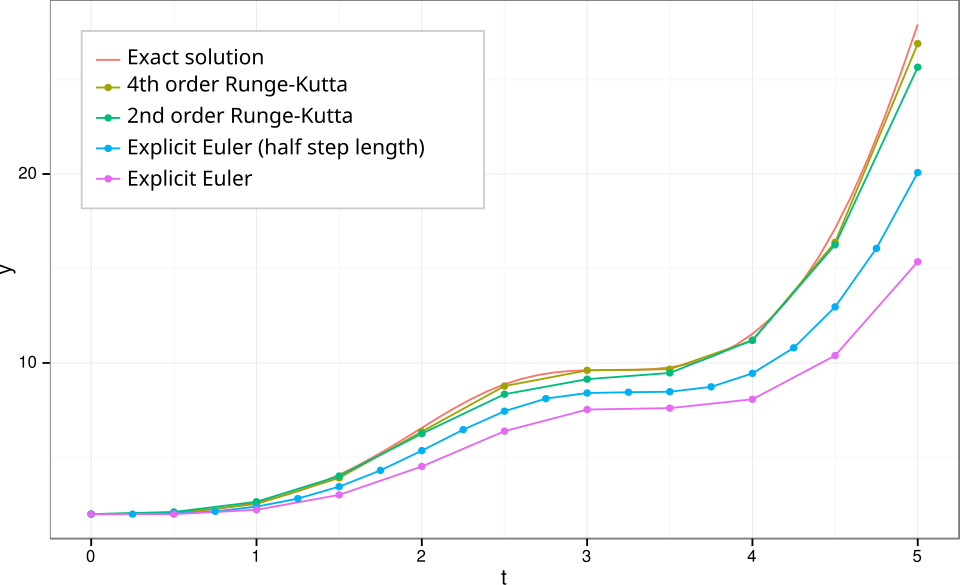
   • Solving ODEs via numerical integration (e.g., Runge-Kutta).
2. Data Science:
   • Estimating probabilities from empirical distributions.
3. Economics:
   • Computing consumer surplus ($\int P(Q)dQ$).
4. Computer Graphics:
   • Rendering curves and surfaces.

A flowchart comparing Trapezoidal, Simpson, and Gaussian quadrature rules. (Image: png image Svchb; svg image tobi; English translation by Prof, CC BY-SA 3.0, via Wikimedia Commons)

Comparative Analysis

table
  | Method               | Pros                                  | Cons                                  | Best For                          |
  |----------------------|---------------------------------------|---------------------------------------|-----------------------------------|
  | Trapezoidal Rule     | Simple, low computation               | Low accuracy ($O(h^2)$)             | Quick estimates                   |
  | Simpson’s Rule       | High accuracy ($O(h^4)$)             | Requires even $n$                   | Smooth functions                  |
  | Romberg Integration  | High precision with few points        | Complex implementation                | High-accuracy needs               |
  | Gaussian Quadrature  | Optimal for given points              | Limited to specific intervals         | Polynomial integrands             |

Exam Tip

Common Pitfalls & Strategies

1. Unit Transformation:

   • Always transform integrals to $[-1,1]$ for Gaussian quadrature.
   • Example: ${\int }_a^{b}f(x)dx=\frac{b-a}{2}{\int }_{-1}^{1}f\left(\frac{(b-a)t+a+b}{2}\right)dt$.

2. Error Calculation:

   • Memorize error bounds for Trapezoidal and Simpson’s rules.
   • For Romberg, recognize that $R_{i,j}$ converges faster than $R_{i,1}$.

3. Numerical Differentiation:

   • Use central differences for interior points to minimize error.
   • For boundary points, use forward/backward differences with adjusted $h$.

4. Exam Questions:

   • Direct Evaluation: Expect 3-4 marks for applying Simpson’s 3/8 or Romberg.
   • Error Analysis: 2 marks for deriving error bounds.
   • Applications: 1 mark for naming a real-world use (e.g., "calculating arc length").

5. Gaussian Quadrature:

   • Know the weights and nodes for 2-point and 3-point formulas.
   • Transform non-standard intervals carefully.

Model Answer Structure

For a 10-mark question on Romberg integration:

1. Step 1 (2 marks): Write the trapezoidal rule for $h$ and $h/2$.
2. Step 2 (3 marks): Compute $R_{1,1}$ and $R_{2,1}$.
3. Step 3 (3 marks): Apply Richardson extrapolation to get $R_{1,2}$.
4. Step 4 (2 marks): Discuss convergence or compare with exact value.

Practice Problems

1. Use Simpson’s 1/3 rule with $n=4$ to evaluate ${\int }_0^1{e}^{-x^2}dx$.
2. Derive the error bound for the trapezoidal rule applied to ${\int }_0^{\pi }\sin xdx$ with $n=4$.
3. Implement a 2-point Gaussian quadrature to approximate ${\int }_0^2{x}^2{e}^{-x}dx$.
4. Given $f(x)=\ln x$, estimate $f^{\prime }(1)$ using central difference with $h=0.1$ and $h=0.01$, then analyze the error.