Introductory MicroeconomicsUnit 814 min read
Perfect Competition: Market Structure, Firm Behavior & Efficiency
Unit 8 of Introductory Microeconomics explores the defining features of perfect competition, how firms and markets behave under this structure, price determination, and its economic efficiency. It contrasts this model with other market structures and applies it to real-world scenarios like agricultural markets and stoc
TAKEAWAYS:
- Perfect competition is defined by homogeneous products, price takers, free entry/exit, and perfect information, creating allocative and productive efficiency.
- Firms maximize profit where MR = MC, and in the long run, P = MR = MC = minimum ATC, ensuring zero economic profit.
- The market supply curve is the horizontal sum of individual firms’ MC curves above AVC, while the demand curve is perfectly elastic.
- Perfect competition leads to Pareto efficiency—no reallocation can make someone better off without harming others—but may underproduce public goods.
- Real-world examples (e.g., Nepal’s NEPSE stock market, Daraz’s seller network, or Kathmandu’s vegetable markets) approximate this model in specific segments.
- Exam focus: Compare perfect competition with monopoly/monopolistic competition; derive equilibrium price/quantity; explain efficiency conditions.
Core Concepts of Perfect Competition
Perfect competition is the benchmark market structure in microeconomics, characterized by:
- Many small firms: No single firm can influence market price.
- Homogeneous products: Identical goods (e.g., wheat, crude oil, or standardized stocks like NEPSE’s Nepal Bank Limited shares).
- Price takers: Firms accept the market price as given.
- Free entry/exit: No barriers to entry or exit (e.g., Daraz sellers can join/leave easily).
- Perfect information: Buyers and sellers know all prices and product details.
Why Does Perfect Competition Exist?
While no market is perfectly competitive, agricultural markets (e.g., Nepal’s maize or rice markets) and financial markets (e.g., NEPSE’s trading of government securities) closely approximate this structure. The key is that no single buyer or seller can manipulate prices.
Market Equilibrium: Price and Quantity Determination
In perfect competition, the market equilibrium price (P)* is where:
How the Market Clears
Individual Firm’s Decision:
- Each firm is a price taker (e.g., a wheat farmer in Pokhara’s vegetable market).
- Marginal Revenue (MR) = Price (P) because firms can sell any quantity at the market price.
- Profit maximization condition: (Marginal Cost).
- Shutdown rule: If , the firm shuts down in the short run.
Market Supply Curve:
- The short-run market supply curve is the horizontal sum of all firms’ MC curves above AVC.
- The long-run supply curve is more elastic because firms can enter/exit freely.
Short-Run vs. Long-Run Equilibrium
| Feature | Short Run | Long Run |
|---|---|---|
| Number of Firms | Fixed | Adjusts (entry/exit) |
| Profit Condition | Can earn economic profit/loss | Zero economic profit (P = min ATC) |
| Market Supply | Inelastic (fixed firms) | Elastic (firms enter/exit) |
| Efficiency | May not be allocatively efficient | Allocatively and productively efficient |
Worked Example: Daraz’s Seller Network (Approximate Perfect Competition)
- Scenario: Daraz allows thousands of small sellers to list identical products (e.g., phone chargers).
- Assumptions:
- Products are homogeneous (no branding differences).
- Sellers cannot collude to raise prices.
- Buyers compare prices instantly (perfect information).
- Outcome:
- If any seller charges above the market price (e.g., Rs. 400 instead of Rs. 350), they lose all sales.
- Equilibrium price = Rs. 350, determined by the intersection of total market demand and supply.
- Long-run result: Only sellers with lowest costs survive (e.g., those using Pokhara-based warehouses).
Firm’s Profit Maximization
In perfect competition:
- Price (P) = Marginal Revenue (MR) = Average Revenue (AR) (perfectly elastic demand).
- Profit (π) = (P – ATC) × Q.
Three Cases in Short Run
- Profit Maximization (P > ATC):
- Firm earns economic profit.
- Example: A Nepalese tea plantation selling at Rs. 200/kg when ATC = Rs. 150/kg.
- Graph:
Break-even (P = ATC):
- Zero economic profit (normal profit).
- Firms stay in the market (no incentive to exit).
Loss Minimization (P < ATC but P > AVC):
- Firm continues operating in the short run.
- Example: A Pokhara-based vegetable seller selling at Rs. 30/kg when ATC = Rs. 40/kg but AVC = Rs. 25/kg.
Shutdown (P < AVC):
- Firm exits the market immediately.
- Example: A Nepalese honey producer selling at Rs. 100/kg when AVC = Rs. 120/kg.
Long-Run Equilibrium: Zero Economic Profit
In the long run:
- Free entry/exit ensures P = min ATC.
- No economic profit (only normal profit).
- Productive efficiency: Firms produce at the lowest possible cost.
- Allocative efficiency: P = MC, ensuring resources go to their highest-valued use.
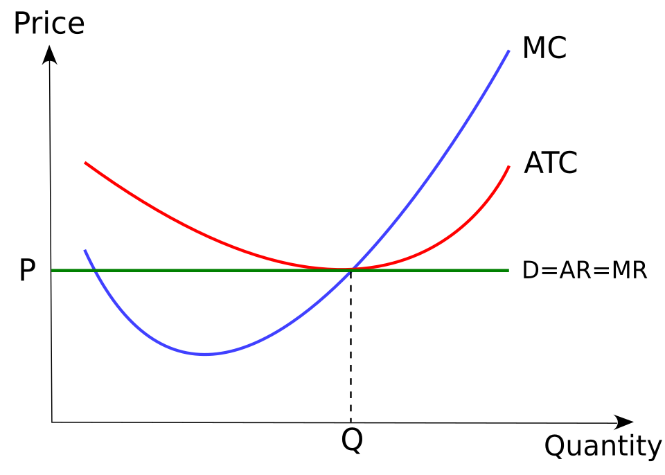 Firm produces where P = MC = min ATC, e.g., a NEPSE stockbroker with zero economic profit. (Image: Costcurve_-_Combined.png: The original uploader was Trampled, CC BY-SA 3.0, via Wikimedia Commons)
Efficiency in Perfect Competition
Perfect competition achieves:
Productive Efficiency:
- Firms produce at the minimum point of ATC.
- Example: NTC’s telecom towers are optimally located to minimize costs.
Allocative Efficiency:
- P = MC, meaning the social benefit (price) equals social cost (MC).
- Example: If Nepal’s electricity tariff (P) equals the marginal cost of generating power (MC), resources are allocated efficiently.
Dynamic Efficiency:
- Innovation and cost reduction drive long-term growth (e.g., Daraz reducing logistics costs).
In the Real World
NEPSE Stock Market (Nepal):
- Idea Used: Homogeneous products (standardized shares) and price takers (investors).
- How: When you buy Nepal Bank Limited shares, the price is determined by market supply and demand, not by any single trader. The market closely resembles perfect competition for blue-chip stocks.
Pokhara’s Vegetable Market (e.g., Satdobato):
- Idea Used: Perfect information and price takers.
- How: Sellers (e.g., potato farmers from Dhading) cannot raise prices above the market-clearing rate (e.g., Rs. 40/kg for potatoes in 2023). If one seller charges Rs. 45/kg, buyers switch to competitors instantly.
Daraz’s Seller Platform:
- Idea Used: Free entry/exit and homogeneous products.
- How: Small businesses in Kathmandu or Pokhara can list products (e.g., Rs. 500 phone chargers) without barriers. If profits are positive, new sellers enter; if losses occur, some exit, driving prices to P = MC in the long run.
Comparison with Other Market Structures
| Feature | Perfect Competition | Monopoly | Monopolistic Competition | Oligopoly |
|---|---|---|---|---|
| Number of Firms | Many | One | Many (differentiated) | Few |
| Product Type | Homogeneous | Unique | Differentiated | Homogeneous/Differentiated |
| Price Control | Price taker | Price setter | Some control | Interdependent pricing |
| Barriers to Entry | None | High | Low | High |
| Profit in LR | Zero | Positive | Zero (but some brand loyalty) | Positive (if barriers exist) |
| Efficiency | Productively & allocatively efficient | Inefficient | Some inefficiency | Mixed efficiency |
| Example (Nepal) | NEPSE stocks, agricultural markets | NTC (telecom monopoly before liberalization) | Kathmandu’s restaurants, Daraz sellers | Ncell/NTC (duopoly), banks |
Advantages and Disadvantages of Perfect Competition
Advantages
✅ Consumer Welfare: Lowest possible prices (P = MC) and high-quality products (due to competition). ✅ Resource Allocation: Efficient use of resources (no waste). ✅ Innovation: Firms must cut costs or improve quality to survive. ✅ Dynamic Efficiency: Long-run adjustments lead to lower costs and better products.
Disadvantages
❌ No Incentive for R&D: Firms earn zero economic profit in LR, so they may underinvest in innovation. ❌ Small Firms Dominate: May lead to market fragmentation (e.g., too many small Daraz sellers). ❌ Public Goods Underproduction: Markets fail to provide non-excludable goods (e.g., clean air, public health). ❌ Price Wars: Can lead to destructive competition (e.g., Ncell vs. NTC cutting prices aggressively).
Exam Tip
Memorize the Key Conditions:
- Short-run equilibrium: , but .
- Long-run equilibrium: .
- Shutdown rule: .
Graphs Are Critical:
- Always draw:
- Market demand and supply curves.
- Individual firm’s MC, AVC, ATC, MR (horizontal line at P).
- Profit/loss rectangles (P – ATC) × Q.
- Label equilibrium points clearly (e.g., , units).
- Always draw:
Compare with Other Structures:
- Monopoly: , , deadweight loss.
- Monopolistic Competition: Differentiated products, excess capacity in LR.
Real-World Applications:
- Agricultural markets (e.g., Nepal’s rice market) ≈ Perfect competition.
- Stock markets (e.g., NEPSE’s government securities) ≈ Perfect competition.
- E-commerce platforms (e.g., Daraz’s seller network) ≈ Monopolistic competition.
Common Exam Questions:
- "Why is a perfectly competitive firm a price taker?" → Because its demand curve is perfectly elastic.
- "What happens if a firm earns economic profit in the short run?" → New firms enter, driving price down to P = ATC in the long run.
- "How does perfect competition ensure efficiency?" → P = MC (allocative) + P = min ATC (productive).
Worked Problem: NEPSE Stock Market Equilibrium
Scenario: In NEPSE, the market for Nepal Bank Limited shares is perfectly competitive. Suppose:
- Market demand for shares:
- Market supply of shares:
- Each share has a marginal cost (MC) of Rs. 50 to trade (brokerage fees).
Questions:
- Find the equilibrium price and quantity.
- If a broker tries to charge Rs. 60 per share, what happens?
- What is the long-run adjustment if brokers earn economic profits?
Solution:
- Equilibrium: Graph:
Broker Charges Rs. 60:
- New quantity demanded: shares.
- Quantity supplied: shares.
- Excess supply: shares → price falls until equilibrium is restored.
Long-Run Adjustment:
- If brokers earn economic profit, new brokers enter (free entry).
- Supply increases, driving price back to P = MC = Rs. 50 (assuming MC is the brokerage cost).
- Result: Zero economic profit in LR, but allocative efficiency is maintained.
Key Takeaways for Exam Success
Draw graphs accurately—examiners check for:
- Correct slopes (demand downward, supply upward).
- Proper labeling of P, Q, MC, ATC, MR.
- Profit/loss areas shaded correctly.
Understand the difference between:
- Short-run (firms can earn profit/loss).
- Long-run (zero economic profit, P = min ATC).
Real-world examples:
- Agricultural markets (e.g., Nepal’s maize market) ≈ Perfect competition.
- Stock markets (e.g., NEPSE’s government bonds) ≈ Perfect competition.
- E-commerce (e.g., Daraz’s generic product sellers) ≈ Monopolistic competition.
Efficiency conditions:
- Perfect competition is the only structure that guarantees both allocative and productive efficiency in the long run.
Final Revision Checklist
✔ Can you derive equilibrium price and quantity for a perfectly competitive market? ✔ Do you know the profit maximization condition () and shutdown rule ()? ✔ Can you compare perfect competition with monopoly/monopolistic competition in a table? ✔ Are you familiar with real-world examples (NEPSE, agricultural markets, Daraz)? ✔ Can you draw and explain the long-run equilibrium where ?
Based on the PU BBA (PU) syllabus for Introductory Microeconomics, unit 8.
Discussion
Loading…