Introductory MicroeconomicsUnit 69 min read
Production: Factors, Functions, Returns, and Short-Run Analysis
Unit 6 of Introductory Microeconomics explores the theory of production, covering production functions, laws of returns, short-run and long-run production decisions, and the role of factors of production in maximizing output.
TAKEAWAYS:
- Production is the process of transforming inputs (land, labor, capital, entrepreneurship) into goods and services using technology and management.
- The law of variable proportions explains how output changes as one input varies while others remain fixed, leading to stages of increasing, diminishing, and negative returns.
- Short-run production is analyzed using total product (TP), average product (AP), and marginal product (MP) curves, which help firms decide optimal input usage.
- Long-run production assumes all inputs are variable, allowing firms to achieve economies of scale by optimizing plant size and technology.
- Real-world firms like Daraz (logistics optimization) and Ncell (network expansion) use production theory to minimize costs and maximize efficiency.
- The production function quantifies how inputs (labor , capital , technology ) combine to produce output .
1. Introduction to Production
Production is the economic process of converting inputs (factors of production) into outputs (goods and services). It is the foundation of economic activity, determining how efficiently resources are used to meet consumer demands.
Factors of Production
Every production process relies on four key inputs:
- Land – Natural resources (e.g., soil, minerals, water).
- Labor – Human effort (skilled/unskilled workers).
- Capital – Man-made tools, machinery, and infrastructure.
- Entrepreneurship – Risk-taking and innovation by business owners.
Real-World Example:
- Nepal’s Agriculture Sector relies heavily on land (terrace farming) and labor (manual harvesting).
- Ncell’s 5G Expansion requires capital (towers, equipment) and entrepreneurship (strategic planning).
2. Production Function
The production function mathematically represents the relationship between inputs and output: Where:
- = Total output
- = Labor input
- = Capital input
- = Technology level
Types of Production Functions:
| Type | Description | Example |
|---|---|---|
| Short-Run | At least one input is fixed (usually capital). | A factory using fixed machinery but varying labor. |
| Long-Run | All inputs are variable; firm can adjust plant size and technology. | Expanding a Daraz warehouse for more orders. |
| Cobb-Douglas | (where ). | Manufacturing firms optimizing labor and capital. |
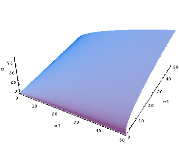 A 3D surface showing how output changes with labor and capital . (Image: CC BY-SA 3.0, via Wikimedia Commons)
3. Laws of Returns (Stages of Production)
When a firm increases one variable input (e.g., labor) while keeping others fixed, output changes in predictable stages:
Three Stages of Production
graph LR
    A["Stage I: Increasing Returns"] -->|"Output rises at an increasing rate"| B["Stage II: Diminishing Returns"]
    B -->|"Output rises but at a decreasing rate"| C["Stage III: Negative Returns"]
C -->|"Output falls as overcrowding occurs"| D["Optimal Output"]| Stage | Total Product (TP) | Marginal Product (MP) | Average Product (AP) | Implication |
|---|---|---|---|---|
| Stage I | Rising at an increasing rate | Positive and rising | Rising | Efficient use of inputs. |
| Stage II | Rising but at a decreasing rate | Positive but falling | Rising then falling | Diminishing returns set in. |
| Stage III | Falls | Negative | Falls | Overuse of input reduces output. |
Worked Example: A Wheat Farm in Nepal
- Fixed Input: 1 hectare of land, irrigation system.
- Variable Input: Labor (farmers).
- Observations:
- 1–3 workers: TP rises rapidly (Stage I).
- 4–6 workers: TP still rises but slower (Stage II).
- 7+ workers: TP falls (Stage III) due to overcrowding.
4. Short-Run Production Analysis
In the short run, firms optimize input usage by analyzing:
- Total Product (TP) – Total output from all inputs.
- Average Product (AP) –
- Marginal Product (MP) – Additional output from one more unit of input:
Key Relationships:
- MP > AP → AP is rising.
- MP = AP → AP is at its maximum.
- MP < AP → AP is falling.
Real-World Application: NTC’s Network Expansion
- NTC adds more technicians (labor) to install fiber optic cables.
- Initially, each new technician increases MP (more cables laid).
- Beyond a point, diminishing returns occur (traffic congestion, delays).
5. Long-Run Production and Returns to Scale
In the long run, all inputs are variable, allowing firms to change plant size and technology.
Returns to Scale
| Type | Description | Example |
|---|---|---|
| Increasing Returns | Doubling inputs more than doubles output. | Google expanding data centers. |
| Constant Returns | Doubling inputs exactly doubles output. | A standardized factory line. |
| Decreasing Returns | Doubling inputs less than doubles output (diseconomies of scale). | Overcrowded Daraz warehouses. |
Economies of Scale (Long-Run Advantages):
- Technical: Larger machines, specialized equipment.
- Managerial: Better division of labor.
- Financial: Bulk purchasing discounts.
- Marketing: Lower per-unit advertising costs.
Worked Example: Pathao’s Ride-Hailing Expansion
- Initially, adding more drivers (increasing returns) reduces average cost per ride.
- At some scale, constant returns are achieved (optimal fleet size).
- Beyond a point, diseconomies may arise (traffic delays, higher wages).
6. Production Possibility Frontier (PPF) and Efficiency
The PPF shows the maximum possible output combinations of two goods given fixed resources.
Key Concepts:
- Attainable vs. Unattainable Points – Points inside/outside the PPF.
- Efficient vs. Inefficient Allocation – Points on vs. inside the PPF.
- Opportunity Cost – The cost of producing one good in terms of the other.
Real-World Example: Nepal’s Trade-Off
- If Nepal allocates more resources to hydropower (capital-intensive), it must reduce agricultural output (labor-intensive).
- Opportunity Cost: For every unit of hydropower, Nepal loses tons of rice.
7. Production in Different Market Structures
| Market Structure | Production Decision | Example |
|---|---|---|
| Perfect Competition | Price taker; produces where . | Wheat farming in Nepal. |
| Monopoly | Profit maximization where . | NTC’s telecom services. |
| Oligopoly | Interdependent pricing (e.g., Ncell vs. NTC). | Mobile network providers. |
In the Real World
Daraz (E-Commerce Logistics)
- Uses production theory to optimize warehouse space and delivery routes.
- Short-run: Hires seasonal workers during sales (Stage II of returns).
- Long-run: Expands warehouses (economies of scale) to reduce per-order costs.
Ncell (Telecom Expansion)
- Capital-intensive production: Installs 5G towers (fixed cost).
- Labor-intensive: Hires technicians (variable cost).
- Faces diminishing returns if too many towers are built in congested areas.
Nepal Rastra Bank (NRB) and Inflation Control
- Studies aggregate production function to predict GDP growth.
- Uses PPF analysis to explain trade-offs between investment and consumption.
Exam Tip
- Memorize the Three Stages of Production – Always draw TP, AP, and MP curves with clear labels.
- Short-Run vs. Long-Run – Short-run has fixed inputs; long-run has all variable.
- Economies of Scale – Explain why firms grow (cost advantages) and when diseconomies occur.
- PPF Questions – Always show opportunity cost and efficiency in diagrams.
- Real-World Links – Relate Daraz’s hiring, NTC’s network expansion, or Nepal’s agriculture to production theory.
- Numerical Problems – Practice calculating MP, AP, and optimal input levels (e.g., "How many workers should a farm hire?").
Common Mistakes to Avoid:
- Confusing short-run (fixed capital) with long-run (all variable).
- Forgetting that MP cuts AP at its maximum.
- Ignoring diseconomies of scale in long-run analysis.
Final Note: Production theory is not just theory—it explains how businesses grow, how costs change, and why some firms fail. Master this unit, and you’ll understand real-world decisions by companies like Daraz, Ncell, and even the Nepal Government’s infrastructure projects.
Based on the PU BBA (PU) syllabus for Introductory Microeconomics, unit 6.
Discussion
Loading…