Computer GraphicsUnit 810 min read
3D Viewing & Projection: Pipelines, Coordinates, Projections & Hidden-Surface Removal
Unit 8 of Computer Graphics covers the 3D viewing pipeline, coordinate systems (world, viewing, normalized device), parallel vs. perspective projection, and hidden-surface removal techniques (back-face culling, painter’s algorithm, area subdivision). Learn how 3D scenes are transformed into 2D images, with visuals of p
TAKEAWAYS:
- The 3D viewing pipeline converts world coordinates → viewing coordinates → normalized device coordinates → screen coordinates via model-view-projection (MVP) transformations.
- Parallel projection preserves parallel lines (used in CAD, floor plans) while perspective projection mimics human vision (used in games, VR).
- Hidden-surface removal ensures only visible surfaces render: back-face culling discards faces away from the viewer; painter’s algorithm sorts polygons by depth.
- Viewing frustum clipping removes objects outside the camera’s view (left, right, near, far planes).
- Orthographic projection (a type of parallel projection) is used in technical drawings; perspective projection uses a projection plane and eye point to create depth.
- Exam focus: Derive projection matrices, explain coordinate systems, and compare parallel vs. perspective projection with real-world examples.
1. The 3D Viewing Pipeline
The 3D viewing pipeline is a sequence of transformations that convert a 3D scene into a 2D image on the screen. It consists of four coordinate systems and three transformation stages:
Coordinate Systems
- World Coordinate System (WCS)
- Objects are defined in this global space (e.g., a cube centered at
(0, 0, 0)). - Real-world analogy: A 3D model in Blender or Unity is designed in world space.
- Objects are defined in this global space (e.g., a cube centered at
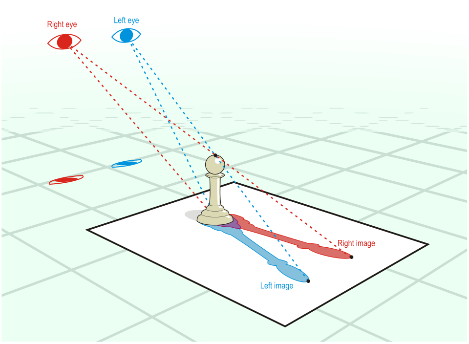 Real-world illustration of how a projection plane and eye point create depth in perspective projection. (Image: CC BY-SA 3.0, via Wikimedia Commons)
Viewing (Eye) Coordinate System (VCS)
- The scene is transformed relative to the camera’s position (eye point) and orientation.
- Transformation: Model-View Matrix (MV) combines translation, rotation, and scaling to position the camera.
- Example: In Pathao’s AR navigation, the camera’s view is aligned with the rider’s perspective.
Normalized Device Coordinate System (NDCS)
- The scene is clipped to a canonical view volume (
[-1, 1]in x, y, z). - Transformation: Projection Matrix (P) converts VCS to NDCS.
- Parallel projection: Uses orthographic projection (no perspective distortion).
- Perspective projection: Uses a projection plane and eye point to simulate depth.
- The scene is clipped to a canonical view volume (
Device Coordinate System (DCS)
- Final coordinates are mapped to the screen resolution (e.g.,
0to1920pixels). - Transformation: Perspective division (
w-coordinate) and viewport scaling.
- Final coordinates are mapped to the screen resolution (e.g.,
graph TD
    A["World Coordinates (WCS)"] -->|"Model-View Matrix (MV)"| B["View Coordinates (VCS)"]
    B -->|"Projection Matrix (P)"| C["Normalized Device Coordinates (NDCS)"]
    C -->|"Perspective Division & Viewport Transform"| D["Device Coordinates (DCS)"]
    D -->|"Screen Resolution (e.g., 0-1920 pixels)"| E["Rendered Image"]
Key Transformations
Model-View Matrix (MV):
- Combines translation, rotation, and scaling to position the camera.
- Example: In Nepal Stock Exchange (NEPSE) 3D visualizations, stocks are rendered in a rotating 3D chart where the camera orbits the data.
Projection Matrix (P):
- Parallel (Orthographic) Projection:
P_{ortho} = \begin{bmatrix} \frac{2}{r-l} & 0 & 0 & -\frac{r+l}{r-l} \\ 0 & \frac{2}{t-b} & 0 & -\frac{t+b}{t-b} \\ 0 & 0 & -\frac{2}{f-n} & -\frac{f+n}{f-n} \\ 0 & 0 & 0 & 1 \end{bmatrix}- Used in CAD software (e.g., AutoCAD) for technical drawings.
- Perspective Projection:
P_{perspective} = \begin{bmatrix} \frac{2n}{r-l} & 0 & \frac{r+l}{r-l} & 0 \\ 0 & \frac{2n}{t-b} & \frac{t+b}{t-b} & 0 \\ 0 & 0 & -\frac{f+n}{f-n} & -\frac{2fn}{f-n} \\ 0 & 0 & -1 & 0 \end{bmatrix}- Used in video games (e.g., GTA V) and VR to create realistic depth.
- Parallel (Orthographic) Projection:
Viewing Frustum Clipping
- The viewing frustum defines the visible volume (left, right, top, bottom, near, far planes).
- Objects outside this volume are clipped (discarded).
- Example: In Daraz’s 3D product viewer, only the visible sides of a shoe are rendered, not the back.
2. Parallel vs. Perspective Projection
| Feature | Parallel Projection | Perspective Projection |
|---|---|---|
| Type | Orthographic, Isometric | Mimics human vision |
| Depth Distortion | None (parallel lines remain parallel) | Objects farther away appear smaller |
| Use Case | CAD, Floor Plans, Technical Drawings | Games, VR, Realistic Rendering |
| Projection Matrix | Orthographic (no division by w) |
Perspective (divide by w after transform) |
| Example | AutoCAD (building blueprints) | Unreal Engine (3D games) |
Worked Example: Orthographic vs. Perspective Projection
Scenario: A cube with vertices at (1,1,1), (1,1,-1), (1,-1,1), etc., is projected with:
Orthographic Projection:
- Viewing volume:
l=-1, r=1, b=-1, t=1, n=1, f=3. - After transformation, all
z-coordinates are scaled but not divided byw. - Result: The cube appears as a rectangle (no depth distortion).
- Viewing volume:
Perspective Projection:
- Same viewing volume, but after transformation, divide
x, y, zbyw. - Result: The cube’s far face appears smaller than the near face.
- Same viewing volume, but after transformation, divide
\text{Orthographic Projection Example:}
\begin{bmatrix}
x' \\
y' \\
z' \\
w'
\end{bmatrix}
=
\begin{bmatrix}
1 & 0 & 0 & 0 \\
0 & 1 & 0 & 0 \\
0 & 0 & -1 & 0 \\
0 & 0 & 0 & 1
\end{bmatrix}
\begin{bmatrix}
1 \\
1 \\
1 \\
1
\end{bmatrix}
=
\begin{bmatrix}
1 \\
1 \\
-1 \\
1
\end{bmatrix}
\rightarrow (x', y', z') = (1, 1, -1) \quad (\text{No division by } w)
\text{Perspective Projection Example:}
\begin{bmatrix}
x' \\
y' \\
z' \\
w'
\end{bmatrix}
=
\begin{bmatrix}
1 & 0 & 0 & 0 \\
0 & 1 & 0 & 0 \\
0 & 0 & -1 & -2 \\
0 & 0 & -1 & 0
\end{bmatrix}
\begin{bmatrix}
1 \\
1 \\
1 \\
1
\end{bmatrix}
=
\begin{bmatrix}
1 \\
1 \\
-3 \\
-1
\end{bmatrix}
\rightarrow (x', y', z') = (-1, -1, 3) \quad (\text{After dividing by } w=-1)
3. Hidden-Surface Removal Techniques
To render only visible surfaces, three main methods are used:
A. Back-Face Culling
- Idea: Discard polygons whose normal vector points away from the viewer.
- Steps:
- Compute the normal vector of the polygon.
- If the dot product of the normal and the view vector is negative, the face is back-facing and discarded.
- Advantage: Fast (used in real-time games like Fortnite).
- Limitation: Only works for closed surfaces (e.g., a cube, not a wireframe).
graph LR
    A["Compute Normal Vector\n(N)"] --> B["Compute View Vector\n(V)"]
    B --> C["Dot Product N·V"]
    C -->|"N·V < 0"| D["Discard (Back-Face)"]
    C -->|"N·V ≥ 0"| E["Render (Front-Face)"]
B. Painter’s Algorithm
- Idea: Sort polygons by depth (z-coordinate) and render from back to front.
- Steps:
- Sort all polygons by their average z-coordinate.
- Render polygons in back-to-front order.
- Advantage: Simple to implement.
- Limitation: Overdrawing occurs if polygons overlap in a way that isn’t depth-sorted (e.g., a spiral staircase).
C. Area Subdivision (Binary Space Partitioning - BSP)
- Idea: Recursively split the scene into front and back regions using planes.
- Steps:
- Choose a split plane (e.g., a polygon’s plane).
- Classify all other polygons as front or back of the plane.
- Recursively process each region.
- Advantage: Efficient for complex scenes (used in Quake III Arena).
- Limitation: Complex to implement.
graph TD
    A["Root Node (Entire Scene)"] --> B["Split Plane (Polygon P)"]
    B --> C["Front Region (Polygons in front of P)"]
    B --> D["Back Region (Polygons behind P)"]
    C --> E["Recursive Split
(Left Subtree)"]
    D --> F["Recursive Split
(Right Subtree)"]
    E -->|"..."| G["Leaf Node (Front)"]
    F -->|"..."| H["Leaf Node (Back)"]
## In the Real World
Pathao’s AR Navigation
- Idea Used: Perspective Projection + Hidden-Surface Removal
- How: The rider’s view in AR shows only the visible parts of the road and buildings, using back-face culling to discard irrelevant surfaces. The projection matrix simulates the rider’s eye position for realistic depth.
NEPSE 3D Stock Visualizations
- Idea Used: Orthographic Projection + Model-View Transformations
- How: Stock price movements are rendered in a 3D rotating chart using orthographic projection to avoid distortion. The model-view matrix adjusts the camera angle for different perspectives.
Daraz’s 3D Product Viewer
- Idea Used: Viewing Frustum Clipping + Perspective Projection
- How: When you rotate a shoe in Daraz’s 3D viewer, only the visible faces are rendered. The viewing frustum ensures no hidden parts (e.g., the sole) are processed unnecessarily, improving performance.
## Exam Tip
Derive Projection Matrices:
- Memorize the orthographic and perspective projection matrices. In exams, you may be asked to derive one from scratch.
- Example: Given
l=-1, r=1, b=-1, t=1, n=1, f=3, write the orthographic projection matrix.
Coordinate System Transformations:
- Explain the purpose of each coordinate system (WCS, VCS, NDCS, DCS) and how they relate to the viewing pipeline.
- Common Mistake: Confusing viewing coordinates (camera-relative) with world coordinates (global).
Parallel vs. Perspective Projection:
- Compare them in a table (as above) and give real-world examples (CAD vs. games).
- Exam Question: "Why does AutoCAD use orthographic projection while GTA V uses perspective?"
Hidden-Surface Removal:
- Back-face culling is the easiest to explain—describe the dot product test.
- For painter’s algorithm, mention the depth-sorting step and its limitation with overlapping polygons.
- Area subdivision is advanced—focus on the recursive splitting concept.
Worked Examples:
- Always show all steps in matrix multiplications (e.g., applying the projection matrix).
- Use simple numbers (e.g., cube vertices at
(±1, ±1, ±1)) to avoid calculation errors.
Visuals in Exams:
- If asked to draw the viewing frustum, label the near, far, left, right, top, bottom planes.
- For projection comparisons, sketch a cube under both orthographic and perspective projections.
Based on the PU BE Computer (PU) syllabus for Computer Graphics, unit 8.
Discussion
Loading…