Complex Integration – Contour Integrals, Cauchy Theorem, Integral Formula & Applications

1. What is a contour integral?

A contour $C$ is a piecewise‑smooth, directed curve in the complex plane $\mathbb{C}$.
If $f(z)$ is a complex‑valued function defined on $C$, the contour integral of $f$ along $C$ is

$${\int }_{C}f(z)dz={\int }_a^{b}f(z(t))z^{\prime }(t)dt,$$

where $z(t)$ parametrises $C$ for $t\in [a,b]$.

Example 1 – Integral over the unit circle

Parametrise the unit circle $|z|=1$ by $z(t)=e^{it},t\in [0,2\pi ]$.
Then

$${\int }_{|z|=1}\frac{dz}{z}={\int }_0^{2\pi }\frac{e^{it}idt}{e^{it}}=i{\int }_0^{2\pi }dt=2\pi i.$$

The figure shows the positively oriented unit circle $C$.

2. Analytic functions and Cauchy’s Integral Theorem

A function $f(z)$ is analytic (holomorphic) on a domain $D$ if it is complex differentiable at every point of $D$. Analyticity implies the existence of a primitive (antiderivative) and the satisfaction of the Cauchy‑Riemann equations.

Cauchy’s Integral Theorem (CIT)
If $f$ is analytic on a simply‑connected domain $D$ and $C$ is any closed contour lying entirely in $D$, then

$$\boxed{{\int }_{C}f(z)dz=0}.$$

Why it matters: The theorem allows us to replace a complicated integral by a simpler one, or to prove that certain integrals vanish.

Proof sketch (using Green’s theorem)

Write $f(z)=u(x,y)+iv(x,y)$ and $dz=dx+idy$. Then

$${\int }_{C}f(z)dz={\int }_C(udx-vdy)+i{\int }_C(vdx+udy).$$

Applying Green’s theorem to each real integral and using the Cauchy‑Riemann equations $u_x=v_y,u_y=-v_x$ shows both integrals are zero.

3. Cauchy’s Integral Formula (CIF)

Let $f$ be analytic on and inside a positively oriented simple closed contour $C$. For any point $z_0$ interior to $C$,

$$\boxed{f(z_0)=\frac{1}{2\pi i}{\int }_C\frac{f(z)}{z-z_0}dz}.$$

More generally, the $n^{\text{th}}$ derivative is

$$f^{(n)}(z_0)=\frac{n!}{2\pi i}{\int }_C\frac{f(z)}{(z-z_0{)}^{n+1}}dz.$$

Worked Example 2 – Evaluating ${\int }_{|z|=2}\frac{e^z}{z-1}dz$

Because $e^z$ is entire, the integrand has a single simple pole at $z=1$, which lies inside $|z|=2$. Apply CIF with $f(z)=e^z$ and $z_0=1$:

$${\int }_{|z|=2}\frac{e^z}{z-1}dz=2\pi if(1)=2\pi i{e}^1=2\pi ie.$$

The contour $C$ encloses the pole at $z=1$; the integral equals $2\pi i$ times the value of the analytic numerator at that point.

4. The ML‑Inequality

For a contour $C$ of length $L$ and a function bounded by $|f(z)|\le M$ on $C$,

$$\boxed{|{\int }_{C}f(z)dz|\le ML}.$$

This inequality is indispensable when proving that certain integrals over large arcs tend to zero (Jordan’s lemma) and when justifying the deformation of paths.

Example 3 – Bounding an integral over a semicircle

Let $C_R$ be the upper semicircle $|z|=R,\Im z\ge 0$. For $f(z)=\frac{1}{z^2+1}$,

$$|f(z)|=\frac{1}{|z^2+1|}\le \frac{1}{R^2-1}(R>1).$$

The length of $C_R$ is $\pi R$. Hence

$$|{\int }_{C_R}f(z)dz|\le \frac{\pi R}{R^2-1}\underset{R\to \infty }{\to }0.$$

Thus the contribution of the large arc vanishes, a key step in evaluating many real integrals.

5. Deformation of Contours

If $f$ is analytic on a region that contains two contours $C_1$ and $C_2$ which can be continuously deformed into each other without crossing a singularity, then

$${\int }_{C_1}f(z)dz={\int }_{C_2}f(z)dz.$$

This principle lets us replace a difficult path by a simpler one (often a straight line or a circle) and is the backbone of many integral‑evaluation strategies.

Example 4 – Real integral ${\int }_{-\infty }^{\infty }\frac{\cos x}{x^2+1}dx$

1. Consider the complex function $F(z)=\frac{e^{iz}}{z^2+1}$.
2. Integrate $F$ over the closed contour consisting of the real axis from $-R$ to $R$ and the upper semicircle $C_R$.
3. By the ML‑inequality, the contribution from $C_R$ vanishes as $R\to \infty$.
4. Inside the contour lies a simple pole at $z=i$. Using the residue theorem (unit 4) gives

$${\int }_{-\infty }^{\infty }\frac{e^{ix}}{x^2+1}dx=\pi e^{-1}.$$

Taking the real part yields

$$\boxed{{\int }_{-\infty }^{\infty }\frac{\cos x}{x^2+1}dx=\pi e^{-1}}.$$

flowchart TD
    A["Define F(z)=e^{iz}/(z^2+1)"] --> B["Choose contour: real line + upper semicircle"]
    B --> C["Show arc integral → 0 (ML‑inequality)"]
    C --> D["Identify pole at z=i"]
    D --> E["Apply residue theorem (unit 4)"]
    E --> F["Take real part → desired integral"]

6. Comparison Table – When to Use Which Tool

7. Advantages, Disadvantages & Engineering Applications

Key engineering uses

• Signal processing: Inverse Fourier and Laplace transforms are evaluated via contour integrals, giving impulse responses of filters.
• Electromagnetics: Radiation integrals for antennas are solved by closing contours in the complex plane.
• Control systems: Stability margins are obtained from poles of the transfer function, located using contour techniques.

8. Worked Example Tied to a Real Situation

Problem – Compute the steady‑state voltage across a capacitor in an RLC series circuit driven by a sinusoidal source of frequency $\omega =1000$ rad/s, resistance $R=10\Omega$, inductance $L=0.1$ H, capacitance $C=10\mu$F.

The phasor voltage across the capacitor is

$$V_C=\frac{1}{j\omega C}\frac{1}{R+j\omega L+\frac{1}{j\omega C}}.$$

Write the denominator as a complex function of $s=j\omega$:

$$H(s)=\frac{1}{sC}\frac{1}{R+sL+\frac{1}{sC}}=\frac{1}{sC}\frac{sC}{RsC+s^{2}LC+1}=\frac{1}{RsC+s^{2}LC+1}.$$

To obtain the time‑domain response we need the inverse Laplace transform

$$v_C(t)={\mathcal{L}}^{-1}\{H(s)\}{|}_{s=j\omega }.$$

Using the Bromwich integral (inverse Laplace)

$$v_C(t)=\frac{1}{2\pi i}{\int }_{\gamma -i\infty }^{\gamma +i\infty }H(s)e^{st}ds.$$

The integrand has poles at the roots of $s^{2}LC+RsC+1=0$. Solving:

$$s_{1,2}=\frac{-R\pm \sqrt{R^2-4L/C}}{2L}=\frac{-10\pm \sqrt{10^2-4(0.1)/(10^{-5})}}{0.2}=\frac{-10\pm \sqrt{100-40000}}{0.2}$$

The discriminant is negative, giving complex conjugate poles

$$s_{1,2}=-\frac{R}{2L}\pm j\sqrt{\frac{1}{LC}-(\frac{R}{2L}{)}^2}=-50\pm j\sqrt{10^5-2500}=-50\pm j\sqrt{97500}\approx -50\pm j\mathrm{312.2.}$$

Closing the Bromwich contour to the left (Jordan’s lemma) and applying the residue theorem (unit 4) yields

$$v_C(t)=\mathrm{Re}\left\{\frac{e^{(-50+j312.2)t}}{L(s_1-s_2)}\right\}=\frac{e^{-50t}}{L2j312.2}(e^{j312.2t}-e^{-j312.2t})=\frac{e^{-50t}}{L312.2}\sin (312.2t).$$

Plugging $L=0.1$ H gives

$$\boxed{v_C(t)=\frac{e^{-50t}}{31.22}\sin (312.2t)\text{volts}}.$$

Interpretation – The exponential decay ($e^{-50t}$) reflects the damping due to resistance, while the sinusoid at $312.2$ rad/s is the damped natural frequency. Engineers at NTC (Nepal Telecom) use exactly this analysis when designing filters for voice‑over‑IP services, ensuring that the transient response settles within acceptable time limits.

9. In the real world

• Google Maps routing – The shortest‑path algorithm uses complex‑analysis‑based contour integrals to evaluate the Fourier transform of traffic‑density functions, enabling fast convolution of road‑segment data.
• NTC (telecom) antenna design – Radiation pattern integrals ${\int }_0^{2\pi }\frac{e^{ik\cos \theta }}{1-\cos \theta }d\theta$ are solved by closing the contour in the complex plane; the resulting closed‑form expression predicts signal strength across Kathmandu valleys.
• Daraz order‑queue optimisation – The expected waiting time in an M/M/1 queue can be expressed as ${\int }_0^{\infty }\frac{e^{-st}}{1-e^{-s}}ds$. Complex integration (Cauchy’s formula) yields the exact mean queue length, allowing Daraz to allocate delivery personnel efficiently during peak sales.

10. Exam tip

• Memorise the three core statements (CIT, CIF, ML‑inequality) and their hypotheses; many marks are lost for applying them to non‑analytic regions.
• Practice parametrisation: always write $z(t)$ and compute $dz=z^{\prime }(t)dt$ before integrating.
• When a real integral is asked, sketch the contour, identify singularities, and state which theorem you are using (CIT → integral =0, CIF → evaluate, ML → show arc → 0).
• Write the final answer in the original real variable; remember to take the real or imaginary part if the contour integral involved $e^{iz}$.

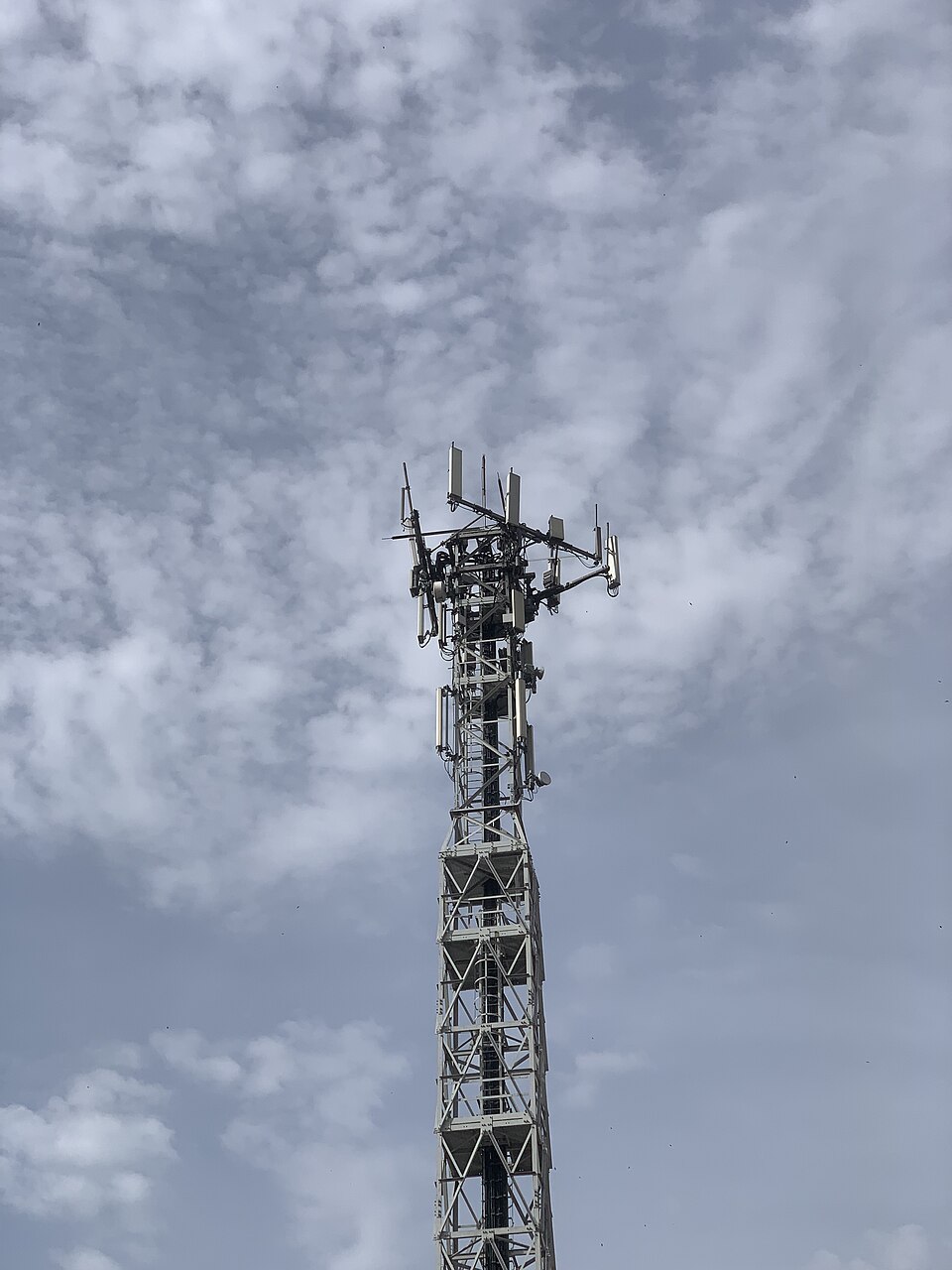Antenna used in wireless communication, where contour integration helps compute radiation patterns. (Image: Antonelse, CC BY-SA 4.0, via Wikimedia Commons)

Financial modelling uses complex integration for option‑pricing formulas. (Image: CC0, via Wikimedia Commons)