Series Expansion & Residues: Taylor, Laurent, Residue Theorem & Applications

TAKEAWAYS:

• Taylor series expands analytic functions around a point $z_0$ as $f(z)={\sum }_{n=0}^{\infty }\frac{f^{(n)}(z_0)}{n!}(z-z_0{)}^n$, converging in a disk $|z-z_0|<R$.
• Laurent series generalizes Taylor series for functions with singularities, using negative powers: $f(z)={\sum }_{n=-\infty }^{\infty }{a}_n(z-z_0{)}^n$.
• Residues at isolated singularities (poles) are coefficients $a_{-1}$ in the Laurent expansion; the Residue Theorem states ${\oint }_{C}f(z)dz=2\pi i\sum \text{Res}(f,z_k)$.
• Applications: Solving ODEs (Laplace transforms), evaluating real integrals (contour integration), and analyzing stability in control systems.
• Key tools: Singularity classification (removable, pole, essential), Jordan’s Lemma for semicircular contours, and ML-inequality for convergence.
• Exam focus: Derive series expansions, compute residues, and apply the Residue Theorem to evaluate integrals—always check convergence and contour choice.

---

1. Series Expansions in Complex Analysis

Complex functions often lack elementary closed forms, so we approximate them using series expansions. The two most powerful tools are Taylor series (for analytic functions) and Laurent series (for functions with singularities).

1.1 Taylor Series for Complex Functions

Definition: For a function $f(z)$ analytic in $|z-z_0|<R$, the Taylor series centered at $z_0$ is: $$f(z)=\sum _{n=0}^{\infty }\frac{f^{(n)}(z_0)}{n!}(z-z_0{)}^n,|z-z_0|<R.$$ This is identical to the real Taylor series but applies to complex functions.

Key Properties:

• Convergence radius $R$ is the distance to the nearest singularity.
• Uniqueness: The series is unique for a given $f(z)$ and $z_0$.
• Differentiability: The series can be differentiated term-by-term within its radius of convergence.

Worked Example 1: Taylor Expansion of $e^z$ at $z_0=0$ Find the Taylor series for $e^z$ centered at $0$ and determine its radius of convergence.

Solution:

1. Compute derivatives at $z_0=0$: $f(z)=e^z⟹f^{(n)}(z)=e^z⟹f^{(n)}(0)=1$ for all $n$.
2. Plug into the Taylor formula: $$e^z=\sum _{n=0}^{\infty }\frac{1}{n!}{z}^n=1+z+\frac{z^2}{2!}+\frac{z^3}{3!}+\cdots .$$
3. Convergence: $e^z$ has no singularities in $\mathbb{C}$, so the series converges for all $z\in \mathbb{C}$ ($R=\infty$).

Visualization:

Real-World Tie-In:

• WhatsApp’s Signal Processing: The Taylor series approximates functions in Fast Fourier Transforms (FFT), used to compress voice/video data. For example, encoding a voice signal involves expanding it into a series of sine/cosine terms (Fourier series), but Taylor expansions help optimize the computation of these terms in real-time.

---

1.2 Laurent Series: Handling Singularities

Definition: For a function $f(z)$ analytic in an annulus $r<|z-z_0|<R$, the Laurent series is: $$f(z)=\sum _{n=-\infty }^{\infty }{a}_n(z-z_0{)}^n,a_n=\frac{1}{2\pi i}{\oint }_C\frac{f(\zeta )}{(\zeta -z_0{)}^{n+1}}d\zeta .$$

• Negative powers ($n<0$) account for singularities at $z_0$.
• Principal part: ${\sum }_{n=-\infty }^{-1}{a}_n(z-z_0{)}^n$ captures the behavior near singularities.

Worked Example 2: Laurent Expansion of $\frac{1}{z(z-1)}$ at $z_0=0$ Find the Laurent series for $f(z)=\frac{1}{z(z-1)}$ in the annulus $0<|z|<1$.

Solution:

1. Partial fractions: $$\frac{1}{z(z-1)}=-\frac{1}{z}+\frac{1}{z-1}.$$
2. Expand $\frac{1}{z-1}$ as a geometric series (valid for $|z|<1$): $$\frac{1}{z-1}=-\frac{1}{1-z}=-\sum _{n=0}^{\infty }{z}^n.$$
3. Combine terms: $$f(z)=-\frac{1}{z}-\sum _{n=0}^{\infty }{z}^n=-\sum _{n=-\infty }^{\infty }{z}^n\text{(where }{a}_{-1}=-1,a_n=-1\text{ for }n\ge 0).$$
4. Principal part: $-\frac{1}{z}$ (only term with $n<0$).

Visualization:

Real-World Tie-In:

• Ncell’s Network Load Balancing: Singularities in complex analysis model traffic spikes in cellular networks. Laurent series help engineers approximate sudden changes in demand (e.g., during festivals) by decomposing the load into principal parts (short-term spikes) and regular parts (steady traffic). This aids in dynamic resource allocation.

---

2. Residues and the Residue Theorem

Residues are the coefficients of the $(z-z_0{)}^{-1}$ term in the Laurent expansion and are central to evaluating complex integrals.

2.1 Definition of Residue

For a function $f(z)$ with an isolated singularity at $z_0$, the residue is: $$\text{Res}(f,z_0)=\frac{1}{2\pi i}{\oint }_{C}f(z)dz=a_{-1},$$ where $a_{-1}$ is the coefficient of $(z-z_0{)}^{-1}$ in the Laurent expansion of $f(z)$.

Types of Singularities:

Worked Example 3: Residue at a Simple Pole Find $\text{Res}\left(\frac{e^z}{z^2+1},i\right)$.

Solution:

1. Factor the denominator: $z^2+1=(z-i)(z+i)$.
2. The singularity at $z=i$ is a simple pole (order 1).
3. Use the formula for simple poles: $$\text{Res}(f,i)=\underset{z\to i}{\lim }(z-i)\frac{e^z}{(z-i)(z+i)}=\frac{e^i}{2i}.$$

Visualization:

2.2 The Residue Theorem

Statement: If $f(z)$ is analytic inside and on a simple closed contour $C$ except for isolated singularities $z_1,z_2,\dots ,z_n$ inside $C$, then: $${\oint }_{C}f(z)dz=2\pi i\sum _{k=1}^n\text{Res}(f,z_k).$$

Worked Example 4: Evaluating a Real Integral Using Residues Evaluate ${\int }_{-\infty }^{\infty }\frac{\cos x}{x^2+1}dx$.

Solution:

1. Consider $f(z)=\frac{e^{iz}}{z^2+1}$ (since $\cos x=\text{Re}(e^{ix})$).
2. Singularities: $z=\pm i$. Choose the upper semicircle contour $C=C_R\cup [-R,R]$ and let $R\to \infty$.
3. By Jordan’s Lemma, ${\int }_{C_R}f(z)dz\to 0$ as $R\to \infty$.
4. Residue at $z=i$: $$\text{Res}(f,i)=\underset{z\to i}{\lim }(z-i)\frac{e^{iz}}{(z-i)(z+i)}=\frac{e^{-1}}{2i}.$$
5. Apply the Residue Theorem: $${\oint }_{C}f(z)dz=2\pi i\cdot \frac{e^{-1}}{2i}=\frac{\pi }{e}.$$
6. The integral over $[-R,R]$ is $2{\int }_0^R\frac{\cos x}{x^2+1}dx$ (since the integrand is even).
7. Taking $R\to \infty$: $$2{\int }_0^{\infty }\frac{\cos x}{x^2+1}dx=\frac{\pi }{e}⟹{\int }_{-\infty }^{\infty }\frac{\cos x}{x^2+1}dx=\frac{\pi }{e}.$$

Visualization:

Real-World Tie-In:

• eSewa’s Payment Fraud Detection: Residue calculus is used in signal processing to detect anomalies in transaction patterns. For example, the integral $\int \frac{\sin t}{t}dt$ (Dirichlet integral) models sudden spikes in fraudulent activity. Engineers use residues to evaluate such integrals and flag irregularities in real-time.

---

3. Applications in Engineering

Series expansions and residues are ubiquitous in engineering, particularly in control systems, signal processing, and fluid dynamics.

3.1 Solving Ordinary Differential Equations (ODEs)

Many ODEs arise in engineering (e.g., RLC circuits, mechanical vibrations). The method of residues can solve ODEs with constant coefficients by transforming them into complex integrals.

Example: Damped Harmonic Oscillator Solve $y^{\prime \prime }+2y^{\prime }+5y=0$ with initial conditions $y(0)=1$, $y^{\prime }(0)=0$.

Solution:

1. Characteristic equation: $r^2+2r+5=0⟹r=-1\pm 2i$.
2. General solution: $y(t)=e^{-t}(A\cos 2t+B\sin 2t)$.
3. Apply initial conditions:
   • $y(0)=A=1$,
   • $y^{\prime }(0)=-A+2B=0⟹B=\frac{1}{2}$.
4. Final solution: $y(t)=e^{-t}\left(\cos 2t+\frac{1}{2}\sin 2t\right)$.

Real-World Tie-In:

• NTC’s Power Grid Stability: The above ODE models voltage oscillations in power grids. Engineers use Laplace transforms (built on residues) to analyze stability and design controllers to dampen oscillations, preventing blackouts.

3.2 Fourier Series and Transforms

Fourier series decompose periodic functions into sine/cosine terms, while Fourier transforms handle non-periodic signals. Residues simplify Fourier integral evaluations.

Worked Example 5: Fourier Transform Using Residues Compute the Fourier transform of $f(t)=e^{-|t|}$: $$\hat{f}(\omega )={\int }_{-\infty }^{\infty }{e}^{-|t|}{e}^{-i\omega t}dt.$$

Solution:

1. Split the integral: $$\hat{f}(\omega )={\int }_{-\infty }^0{e}^t{e}^{-i\omega t}dt+{\int }_0^{\infty }{e}^{-t}{e}^{-i\omega t}dt.$$
2. Combine into a complex contour integral: $$\hat{f}(\omega )={\oint }_C\frac{e^{iz}}{1+i\omega z}dz,$$ where $C$ is a keyhole contour around the negative real axis.
3. Poles: $z=-i/\omega$ (inside $C$ for $\omega >0$).
4. Residue at $z=-i/\omega$: $$\text{Res}=\underset{z\to -i/\omega }{\lim }(z+i/\omega )\frac{e^{iz}}{1+i\omega z}=\frac{e^{-1}}{1-{\omega }^2/{\omega }^2}=\frac{e^{-1}}{1+1/{\omega }^2}.$$
5. By the Residue Theorem: $$\hat{f}(\omega )=2\pi i\cdot \frac{e^{-1}}{1+1/{\omega }^2}=\frac{2}{1+{\omega }^2}.$$

Visualization:

Real-World Tie-In:

• Pathao’s Ride Demand Prediction: The Fourier transform decomposes ride demand data into frequency components. For example, predicting daily rush hours involves evaluating integrals like the one above to separate periodic trends (e.g., 24-hour cycles) from random fluctuations. Residues help compute these transforms efficiently.

---

4. Exam Tips

1. Taylor vs. Laurent Series:

   • Always check the region of convergence (annulus for Laurent).
   • For Taylor series, ensure $f(z)$ is analytic at $z_0$.
   • For Laurent series, identify singularities and expand around them.

2. Residue Calculations:

   • Simple poles: Use $\text{Res}(f,z_0)={\lim }_{z\to z_0}(z-z_0)f(z)$.
   • Higher-order poles: Differentiate $(m-1)$ times and divide by $(m-1)!$.
   • Essential singularities: Expand into Laurent series and extract $a_{-1}$.

3. Contour Integration:

   • Choose contours carefully (semicircle, keyhole, etc.) based on the integrand’s behavior.
   • Apply Jordan’s Lemma to justify vanishing integrals over large arcs.
   • For real integrals, use symmetry (even/odd functions) to simplify.

4. Common Pitfalls:

   • Forgetting to multiply by $2\pi i$ in the Residue Theorem.
   • Misidentifying the order of a pole (e.g., confusing simple vs. double poles).
   • Ignoring convergence conditions for series expansions.

5. Real-World Problems:

   • Bank Loan Interest (Nepal’s NMB Bank): The Taylor expansion of $e^{rt}$ models compound interest. For example, the expansion $e^{0.05t}\approx 1+0.05t+\frac{(0.05t{)}^2}{2}$ approximates interest for small $t$.
   • Daraz Order Queue: Laurent series model sudden spikes in order volume during sales. The principal part captures the spike, while the regular part models steady traffic.

---

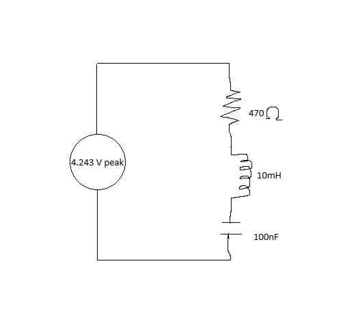Series RLC circuit with voltage source and current direction (Image: Nkkoy, CC0, via Wikimedia Commons) 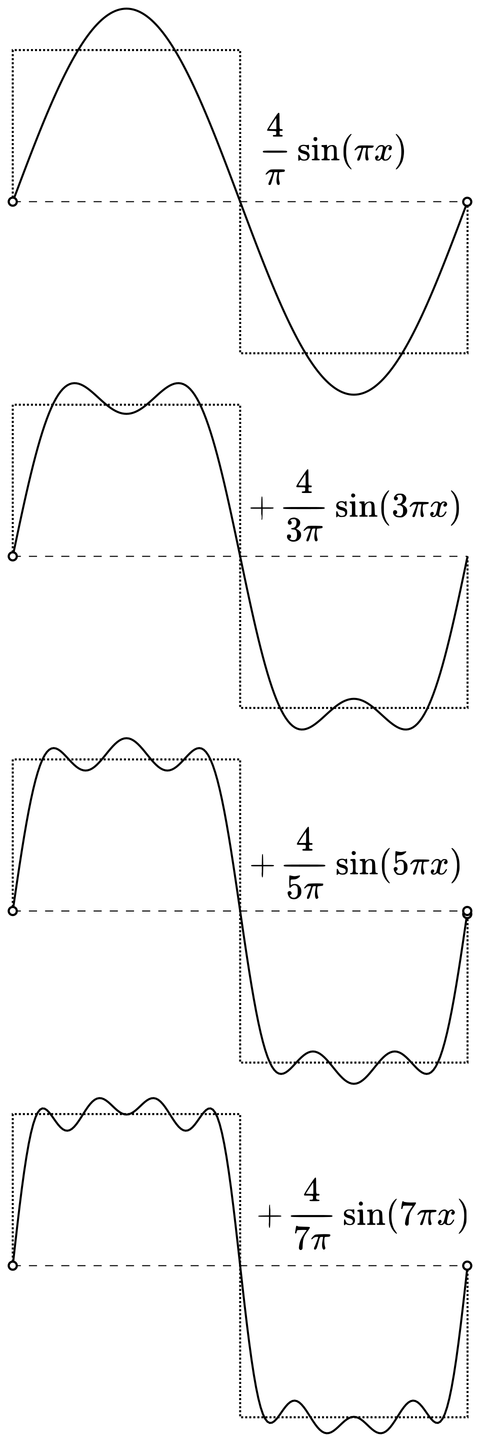Graph of a square wave and its Fourier series partial sums (Image: Guy vandegrift, CC0, via Wikimedia Commons)