Geographical Information SystemUnit 57 min read
Vector Data Analysis: Topology, Overlay, Network & Buffer Techniques
Unit 5 of Geographical Information System explores how vector data (points, lines, polygons) are analyzed in GIS using topological operations, spatial overlays, network analysis, and buffer techniques—essential for real-world applications like route optimization, land-use planning, and disaster management.
Core Concepts of Vector Data Analysis
Vector data represents geographic features as discrete objects (points, lines, polygons) with attributes. Unlike raster data, vector analysis focuses on topological relationships (how features connect, overlap, or relate spatially) and geometric operations (e.g., buffering, overlay). This unit covers four key techniques:
1. Topology in GIS
Topology defines how vector features spatially relate to each other (e.g., adjacency, connectivity, containment). It ensures data integrity during editing and analysis.
- Key topological rules:
- Adjacency: Two polygons share a common boundary (e.g., Kathmandu and Lalitpur districts).
- Connectivity: Lines (roads, rivers) meet at nodes (intersections, junctions).
- Containment: A polygon (e.g., a village) lies entirely within another (e.g., a district).
graph TD
    A["Polygon A (District)"] -->|"contains"| B["Polygon B (Village)"]
    C["Line 1 (Road)"] -->|"connects to"| D["Node (Intersection)"]
    D --> E["Line 2 (Road)"]
    B -->|"adjacent to"| F["Polygon C (Village)"]
Why topology matters:
- Prevents gaps or overlaps in datasets (e.g., a road network where two streets meet at a node).
- Enables advanced analyses like network routing (e.g., Pathao’s delivery optimization) or territorial disputes (e.g., land boundary conflicts).
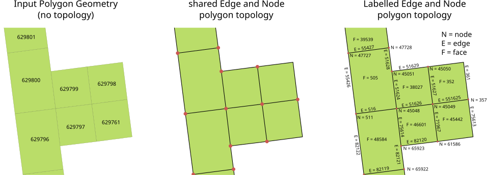 Shows adjacency, connectivity, and containment rules in a vector dataset. (Image: Arbeck, CC BY 4.0, via Wikimedia Commons)
2. Spatial Overlay Analysis
Overlay combines multiple vector layers to answer "what’s here?" questions. Common methods:
- Intersection: Identifies features common to all input layers (e.g., "Which areas are both flood-prone and near schools?").
- Union: Merges all features from input layers (e.g., combining district boundaries with election zones).
- Identity: Retains features from one layer that overlap with another (e.g., "Which roads pass through protected forests?").
Worked Example: Kathmandu Traffic Congestion
Problem: Identify high-traffic roads near schools to plan bypass routes. Steps:
- Input Layers:
- Layer 1: Road network (vector lines) with traffic volume data.
- Layer 2: School locations (points) within 500m of roads.
- Overlay: Use a buffer (500m radius around schools) + intersection with roads.
- Output: Roads overlapping the buffer are flagged for congestion analysis.
flowchart LR
    A["Road Network Layer"] -->|"Buffer 500m"| B["School Buffer Zones"]
    B -->|"Intersection"| C["High-Traffic Roads Near Schools"]
    C --> D["Propose Bypass Routes"]
3. Network Analysis
Analyzes connected vector data (e.g., roads, rivers, utilities) to solve pathfinding, connectivity, or service-area problems. Key operations:
- Shortest path: Finds the quickest route (e.g., Pathao’s delivery optimization).
- Service area: Defines regions accessible within a time/distance (e.g., "Which areas are within 30 minutes of an NTC substation?").
- Closest facility: Locates nearest services (e.g., "Find the nearest blood bank during an emergency").
Real-World Example: Daraz Delivery Routes
Daraz uses network analysis to:
- Model roads as a graph (nodes = intersections, edges = road segments with travel times).
- Apply shortest-path algorithms (e.g., Dijkstra’s) to optimize delivery routes.
- Avoid traffic hotspots (e.g., roads near schools during school hours).
4. Buffer Analysis
Creates zones at a fixed distance from features (points, lines, polygons). Used for:
- Proximity analysis: "Which villages are within 2km of a river?" (flood risk).
- Regulation zones: "No construction within 100m of a protected forest."
- Service areas: "Which areas are within 5km of an eSewa kiosk?"
Worked Example: NEPSE Stock Exchange Zones
Problem: Identify high-value properties near the NEPSE building for potential acquisitions. Steps:
- Create a 1km buffer around the NEPSE building (polygon).
- Overlay with a land-value raster layer (from NEB).
- Extract properties with values > Rs. 5 million within the buffer.
Comparing Vector Analysis Techniques
| Technique | Input Data | Output | Example Use Case |
|---|---|---|---|
| Topology | Adjacent polygons/lines | Validated data (no gaps/overlaps) | Land boundary disputes (e.g., India-Nepal) |
| Overlay | Multiple vector layers | Combined features (intersection/union) | Flood risk mapping (rivers + buildings) |
| Network Analysis | Connected lines (roads, rivers) | Optimal paths/service areas | Pathao delivery routes |
| Buffer | Points/lines/polygons | Distance-based zones | School safety zones (500m no-construction) |
In the Real World
eSewa & Khalti:
- Use buffer analysis to locate merchant kiosks within 1km of high-density user areas (identified via mobile data).
- Network analysis optimizes payment routing to reduce transaction delays.
NTC (Nepal Telecommunications):
- Overlay analysis combines terrain data (raster) with tower locations (vector) to predict signal coverage gaps.
- Topology ensures no overlaps in tower service areas to avoid interference.
Daraz Logistics:
- Shortest-path algorithms (network analysis) reduce delivery times by 20% by avoiding congested routes near schools during peak hours.
- Buffer zones around warehouses define safe loading/unloading areas.
Nepal Police Traffic Management:
- Overlay of accident hotspots (points) with road networks (lines) identifies high-risk intersections for traffic lights.
Advantages and Limitations
Advantages:
- Precision: Vector data is exact (e.g., a road’s exact length vs. raster’s pixel approximation).
- Scalability: Works from local (e.g., a village map) to national (e.g., Nepal’s topography).
- Attribute-rich: Each feature carries metadata (e.g., a road’s width, material, or traffic rules).
Limitations:
- Complexity: Topological errors (e.g., dangling nodes) require manual fixes.
- Data volume: High-resolution vector datasets (e.g., LiDAR-derived contours) consume storage.
- Overlay cost: Combining large layers (e.g., Nepal’s 753 municipalities) is computationally intensive.
Exam Tip
Diagrams are mandatory: Always draw a Mermaid flowchart or labelled diagram for overlay/network/buffer questions. Examiners deduct marks for missing visuals.
- Example: For a buffer question, show:
- Input feature (point/line).
- Buffer zone (dashed circle).
- Overlay result (highlighted area).
- Example: For a buffer question, show:
Real-world tie-ins: Link answers to Nepalese contexts (e.g., "Use NTC’s tower placement as an example of network analysis").
Topology traps:
- Avoid assuming features are topologically clean. State: "Assuming the road network has no dangling nodes..."
Units matter: Buffer distances should be in meters/km, not pixels (raster units).
Common mistakes:
- Confusing union (all features merged) vs. intersection (only overlapping features).
- Forgetting to project data into the same coordinate system before overlay (e.g., UTM Zone 44N for Nepal).
Key Formulae to Memorize:
- Buffer distance = (e.g., 500m buffer).
- Network cost = (for shortest-path calculations).
- Overlay area = (simplified as "shared polygon area").
Based on the TU BIT syllabus for Geographical Information System (BIT355), unit 5.
Discussion
Loading…