Introductory MicroeconomicsUnit 713 min read
Costs: Types, Short-run vs. Long-run, Cost Curves & Decision-Making
Unit 7 of Introductory Microeconomics explores the theory of production costs, distinguishing between short-run and long-run costs, analyzing cost curves (AFC, AVC, MC, AC), and applying cost concepts to firm decision-making under different market structures.
TAKEAWAYS:
- Costs are classified into fixed (FC), variable (VC), total (TC), average (AC), and marginal (MC) costs, each playing a distinct role in production decisions.
- Short-run costs involve at least one fixed factor (e.g., factory size), while long-run costs allow all factors to vary, leading to economies of scale.
- Cost curves (AFC, AVC, MC, AC) intersect at key points (e.g., MC cuts AC at its minimum), guiding profit-maximizing output levels.
- Shutdown rule: A firm should continue operating if P ≥ AVC; otherwise, it should shut down in the short run.
- Long-run equilibrium occurs where AC is minimized, and firms earn normal profits (zero economic profit).
- Real-world applications include pricing strategies (e.g., Daraz’s dynamic pricing), cost control in banks (e.g., NMB’s loan interest calculations), and government regulations (e.g., NTC’s cost-based tariffs).
1. Definitions and Classifications of Costs
Costs are the expenses incurred by firms to produce goods and services. They are categorized based on their behavior and the time horizon of production decisions.
Types of Costs
| Type | Definition | Example (Nepal Context) |
|---|---|---|
| Fixed Cost (FC) | Costs that do not change with output (e.g., rent, machinery depreciation). | Rent paid by Daraz’s warehouse in Kathmandu, regardless of how many orders it processes. |
| Variable Cost (VC) | Costs that vary directly with output (e.g., raw materials, labor). | Pathao’s driver wages increase as the number of rides rises. |
| Total Cost (TC) | Sum of fixed and variable costs: TC = FC + VC. | Ncell’s total cost for producing 10,000 SIM cards includes factory rent (FC) + plastic (VC). |
| Average Cost (AC) | Total cost per unit of output: AC = TC/Q. | NMB Bank’s average cost per loan: ₹50,000 total cost for 10 loans → AC = ₹5,000/loan. |
| Marginal Cost (MC) | Additional cost of producing one more unit: MC = ΔTC/ΔQ. | eSewa’s marginal cost of processing one more transaction: ₹2 (server + labor). |
2. Short-Run vs. Long-Run Costs
The time horizon determines whether a firm can adjust all inputs.
Short-Run Costs
- At least one factor is fixed (e.g., factory size, machinery).
- Law of Diminishing Returns: As variable inputs (e.g., labor) increase, marginal product eventually declines.
- Example: A Kathmandu traffic route (fixed road width) sees congestion as more cars (variable input) enter.
- Visual:
flowchart TD
  A["Increase Labor (Variable Input)"] --> B["Marginal Product ↑"]
  B --> C["Marginal Product ↓ (Diminishing Returns)"]
  C --> D["Total Output ↑ but at decreasing rate"]
Long-Run Costs
- All factors are variable (e.g., firm can build a new factory).
- Economies of Scale: Long-run average costs fall as output expands due to specialization, bulk purchasing, or technology.
- Example: Nepal’s cement industry (e.g., Shree Cement) reduces per-unit costs by expanding production.
- Diseconomies of Scale: Beyond a point, coordination costs rise (e.g., NTC’s bureaucracy slowing efficiency).
- Visual:
3. Cost Curves and Their Relationships
Cost curves illustrate how costs behave as output changes. Key curves:
- Average Fixed Cost (AFC): Declines continuously as output rises (FC spread over more units).
- Example: NMB Bank’s AFC per loan drops from ₹10,000 (10 loans) to ₹5,000 (20 loans).
- Average Variable Cost (AVC): U-shaped due to diminishing returns.
- Marginal Cost (MC): Typically U-shaped; intersects AC at its minimum.
- Average Total Cost (AC): Sum of AFC and AVC; also U-shaped.
- Q = 500 units* (where MC = AC).
- AFC = ₹20/unit, AVC = ₹30/unit, AC = ₹50/unit at Q = 500 (for a hypothetical Daraz delivery firm).
Key Relationships
- MC cuts AC at its minimum: This is the profit-maximizing output level.
- Example: Pathao’s optimal number of drivers is where MC of hiring one more driver equals AC.
- AFC declines but never touches MC or AVC.
4. Shutdown Rule and Profit Maximization
Firms decide whether to produce or shut down based on costs and revenue.
Short-Run Shutdown Decision
| Condition | Decision | Example |
|---|---|---|
| P ≥ AVC | Continue operating (cover variable costs). | Daraz delivers orders even if price = ₹500 (AVC = ₹400). |
| P < AVC | Shut down (cannot cover variable costs). | NTC stops a power plant if electricity price < ₹5/kWh (AVC). |
| P ≥ AC | Earn economic profit. | NMB Bank charges 12% interest > AC of ₹10% on loans. |
| P = AC | Normal profit (zero economic profit). | Khalti’s transaction fee = AC of processing payments. |
- AC curve (U-shaped), AVC curve (below AC), MC curve (cutting AC at minimum).
- Price lines: P1 (above AVC, operate), P2 (below AVC, shut down).
- Label: "NTC’s shutdown price for a hydropower plant: ₹6/MWh (AVC)."
5. Long-Run Equilibrium and Minimum Efficient Scale (MES)
In the long run, firms adjust all inputs to minimize costs.
Key Concepts
- Minimum Efficient Scale (MES): Smallest output where LRAC is minimized.
- Example: Nepal’s cement plants achieve MES at 500,000 tons/year (e.g., Shree Cement).
- Constant Returns to Scale: LRAC remains flat (e.g., digital firms like eSewa).
- Increasing Returns: LRAC falls (e.g., Ncell’s call centers expanding).
- Decreasing Returns: LRAC rises (e.g., NTC’s overstaffed bureaucracy).
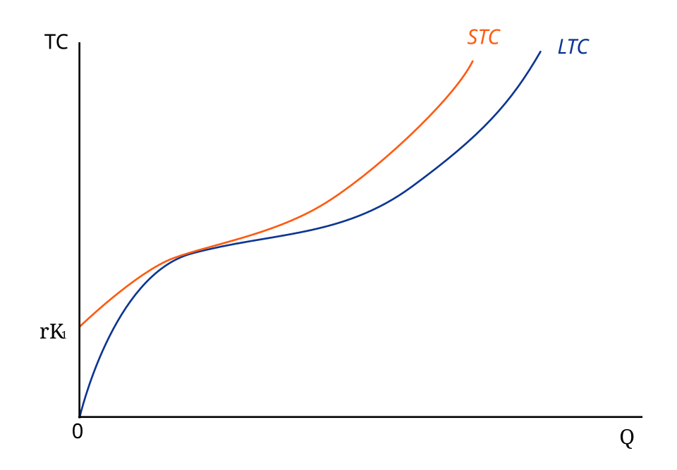 A graph with: (Image: Kwj2772, CC BY-SA 4.0, via Wikimedia Commons)
- LRAC curve (U-shaped).
- SRAC curves (above LRAC, tangent at MES).
- Label: "MES for a Pathao fleet: 1,000 drivers where LRAC = ₹500/day."
6. Real-World Applications
1. Dynamic Pricing by Daraz
- Idea Used: Marginal Cost (MC) and Price Elasticity.
- How: Daraz adjusts prices based on demand (e.g., higher prices during Dashain sales when MC rises due to shipping costs).
- Example:
- MC of delivering a product: ₹200 (peak season) vs. ₹100 (off-season).
- Price: ₹1,500 (peak) vs. ₹1,200 (off-season) to maximize profit.
2. Bank Loan Interest Rates (NMB, Global IME)
- Idea Used: Average Cost (AC) and Risk Premium.
- How: Banks set interest rates to cover AC of lending + profit.
- Example: A ₹10 lakh loan with:
- AC = 8% (salaries, branch rent, default risk).
- Interest rate = 12% (includes 4% profit margin).
- Visual:
- Example: A ₹10 lakh loan with:
3. NTC’s Electricity Tariffs
- Idea Used: Average Variable Cost (AVC) and Regulatory Pricing.
- How: NTC sets tariffs based on AVC of generation + fixed costs.
- Example: If AVC = ₹5/kWh and FC = ₹2/kWh, NTC charges ₹7/kWh to break even.
- Shutdown Rule: If market price < AVC, NTC may reduce supply (e.g., during monsoon when hydropower is cheap).
4. Kathmandu Traffic Congestion (Public Goods vs. Private Costs)
- Idea Used: Marginal Social Cost (MSC) vs. Private Cost.
- How: Traffic jams impose external costs (e.g., pollution, time loss) not reflected in private MC (driver’s cost).
- Example:
- Private MC of driving: ₹50 (fuel + toll).
- MSC: ₹150 (includes congestion delay for others).
- Solution: Toll roads or odd-even schemes internalize MSC.
- Example:
7. Worked Example: Profit Maximization for a Local Bakery
Scenario: A bakery in Pokhara sells roti with the following cost structure:
- FC (rent, oven): ₹5,000/month.
- VC per roti: ₹10 (flour, labor).
- Price (P): ₹20/roti.
Questions:
- What is the profit-maximizing quantity?
- Should the bakery shut down if P = ₹15?
- What is the break-even price?
Solution:
Profit Maximization:
- MC = VC per additional roti = ₹10.
- MR = P = ₹20 (perfect competition).
- Rule: Produce where MC = MR → Q = 500 rotis/month.
- AC = (FC + VC)/Q = (₹5,000 + ₹5,000)/500 = ₹20/roti.
- Profit = (P − AC) × Q = (₹20 − ₹20) × 500 = ₹0 (normal profit).
Shutdown Decision at P = ₹15:
- AVC = VC/Q = ₹10/roti.
- P (₹15) > AVC (₹10) → Continue operating (cover variable costs).
- Loss: (AVC − P) × Q = (₹10 − ₹15) × 500 = ₹2,500 loss.
Break-Even Price:
- Break-even when P = AC.
- AC = ₹20/roti (from above).
- If P < ₹20, the bakery incurs losses.
- MC = ₹10 (horizontal line).
- AC = U-shaped, minimum at Q = 500, AC = ₹20.
- P = ₹20 (tangent to AC at Q = 500).
- Label: "Profit-maximizing output for Pokhara Roti House."
8. Comparison Table: Short-Run vs. Long-Run Costs
| Feature | Short-Run Costs | Long-Run Costs |
|---|---|---|
| Adjustable Factors | At least one fixed (e.g., factory size). | All factors variable. |
| Time Horizon | Days to months. | Years. |
| Cost Curves | SRAC (U-shaped), AFC declines. | LRAC (U-shaped), economies/diseconomies. |
| Decision Rule | Shut down if P < AVC. | Exit if P < AC; enter if P > AC. |
| Example (Nepal) | NTC adjusting hydropower output daily. | Ncell building a new tower in 2 years. |
9. Advantages and Disadvantages of Cost Analysis
| Advantages | Disadvantages |
|---|---|
| Helps firms maximize profit by identifying optimal output. | Assumes perfect information (real firms face uncertainty). |
| Guides pricing strategies (e.g., Daraz’s dynamic pricing). | Ignores externalities (e.g., pollution costs in Kathmandu traffic). |
| Useful for government regulation (e.g., NTC’s tariff setting). | Fixed costs can mislead short-run decisions (e.g., keeping unprofitable routes). |
| Explains economies of scale (e.g., Nepal’s cement industry). | Long-run adjustments take time (e.g., Ncell expanding infrastructure). |
10. Exam Tip
How This Unit is Examined (PU Pattern)
Definitions (5 marks):
- Expect questions on FC, VC, MC, AC, SRAC, LRAC, MES, shutdown rule.
- Example Question:
"Define ‘marginal cost’ and explain why it intersects the average cost curve at its minimum point."
Graph-Based Questions (10 marks):
- Draw and label cost curves (AFC, AVC, MC, AC) with equilibrium points.
- Example Question:
"Given a firm’s cost curves, determine the profit-maximizing output if P = ₹50. Should the firm shut down if P = ₹30? Justify with reference to AVC."
Numerical Problems (10 marks):
- Calculate TC, AC, MC from given data.
- Apply the shutdown rule or profit-maximization rule.
- Example Question:
"A firm has FC = ₹10,000 and VC = ₹2Q. If P = ₹50, find: (a) Profit-maximizing output. (b) Whether the firm should shut down if P = ₹20."
Real-World Applications (5 marks):
- Relate concepts to Nepalese firms (e.g., Daraz, NTC, banks).
- Example Question:
"How does the concept of ‘economies of scale’ help explain why Nepal’s cement industry has fewer but larger firms?"
Short Notes (5 marks):
- Key terms: "Law of diminishing returns," "minimum efficient scale," "shutdown point."
- Example Question:
"Explain the relationship between MC and AC with a diagram."
Marks Distribution (Typical PU Exam)
| Question Type | Marks | Weightage |
|---|---|---|
| Definitions | 5 | 10% |
| Graphs | 10 | 20% |
| Numerical Problems | 10 | 20% |
| Real-World Applications | 5 | 10% |
| Short Notes | 5 | 10% |
| Case Study (e.g., NTC tariffs) | 15 | 30% |
Common Mistakes to Avoid
- Ignoring the shutdown rule: Always check P vs. AVC for short-run decisions.
- Mislabeling curves: Remember AFC declines, AVC is U-shaped, MC cuts AC at minimum.
- Forgetting long-run adjustments: In the long run, firms can enter/exit if P ≠ AC.
- Overlooking real-world ties: PU exams love Nepalese examples (e.g., Daraz, NTC, banks).
Final Tip:
"Draw the graph first!" – Cost curve questions are worth 20% of marks. Sketch AFC, AVC, MC, AC and label equilibria before writing explanations. For numerical problems, show all steps (e.g., TC = FC + VC, AC = TC/Q, MC = ΔTC/ΔQ). Use Nepalese examples (e.g., Daraz, NTC, banks) to stand out in case studies.
Based on the PU BBA (PU) syllabus for Introductory Microeconomics, unit 7.
Discussion
Loading…