Data Science and AnalyticsUnit 610 min read
Predictive Modelling: Algorithms, Evaluation & Applications
Unit 6 of Data Science and Analytics explores supervised learning techniques for forecasting future outcomes, covering regression, classification, model evaluation metrics, and real-world deployment challenges.
TAKEAWAYS
- Predictive modelling uses historical data to forecast outcomes via supervised learning (regression for continuous values, classification for discrete labels).
- Key algorithms include linear regression, decision trees, SVM, and neural networks, each suited to different data structures and problem types.
- Model performance is evaluated using accuracy, precision, recall, RMSE, and ROC curves, with trade-offs between bias and variance.
- Feature engineering (scaling, encoding, selection) and hyperparameter tuning critically impact model accuracy.
- Real-world applications range from fraud detection (Khalti) to demand forecasting (Daraz) and traffic prediction (Pathao).
1. What is Predictive Modelling?
Predictive modelling is a supervised machine learning technique that uses historical data to predict future outcomes. Unlike descriptive analytics (which summarizes past data), predictive models forecast trends, classify categories, or estimate values based on patterns.
Key Components
graph LR
    A["Historical Data"] --> B["Feature Selection"]
    B --> C["Model Training"]
    C --> D["Algorithm Selection"]
    D --> E["Prediction"]
E --> F["Evaluation & Deployment"]- Input (X): Features (independent variables) like age, income, or weather conditions.
- Output (Y): Target variable (dependent variable) like house price, disease risk, or customer churn.
- Model: Learns the mapping from training data.
Types of Predictive Models
| Task | Output Type | Example Algorithms | Use Case |
|---|---|---|---|
| Regression | Continuous (numeric) | Linear Regression, Polynomial Regression | House price prediction |
| Classification | Discrete (labels) | Logistic Regression, Decision Trees, SVM | Spam detection (e.g., Khalti alerts) |
| Time Series | Sequential data | ARIMA, LSTM, Prophet | Stock price forecasting (NEPSE) |
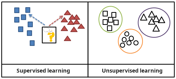 Contrast between labelled (predictive) and unlabelled (descriptive) data. (Image: Balkiss.hamad, CC BY-SA 4.0, via Wikimedia Commons)
2. Regression: Predicting Continuous Values
Regression models predict numeric outputs (e.g., temperature, sales, stock prices). The most common type is linear regression, which assumes a linear relationship between features and target.
How Linear Regression Works
The model fits a line to data using the least squares method, minimizing the sum of squared errors (SSE): where:
- : Actual value
- : Predicted value ()
Worked Example: Daraz Sales Forecasting
Problem: Predict monthly sales for a Daraz seller based on past data (ad spend, promotions, seasonality). Data:
| Month | Ad Spend ($) | Promotions (Y/N) | Sales (Units) |
|---|---|---|---|
| Jan | 500 | N | 200 |
| Feb | 800 | Y | 450 |
| ... | ... | ... | ... |
Model: Output:
- If ad spend = $1000 and no promotion, predicted sales = 320 units (with 95% confidence interval: 280–360).
Limitations:
- Assumes linearity (use polynomial regression for curves).
- Sensitive to outliers (try robust regression).
3. Classification: Predicting Discrete Labels
Classification models assign input data to categories (e.g., spam/not spam, fraud/legit). Key algorithms:
A. Logistic Regression (Binary Classification)
- Uses sigmoid function to output probabilities (0 to 1):
- Decision boundary: → Class 1.
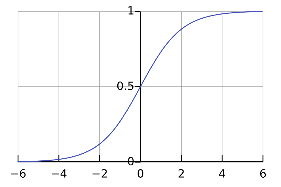 Showing probability threshold at 0.5. (Image: Qef (talk), Public domain, via Wikimedia Commons)
B. Decision Trees
- Splits data into branches based on feature thresholds (e.g., "Income > $50K?").
- Advantages: Interpretable, handles non-linear data.
- Disadvantages: Prone to overfitting (mitigated by pruning).
C. Support Vector Machines (SVM)
- Finds the optimal hyperplane separating classes (works well in high dimensions).
- Kernel trick: Maps data to higher dimensions for non-linear separation.
Comparison Table:
| Algorithm | Best For | Pros | Cons |
|---|---|---|---|
| Logistic Regression | Binary classification | Simple, interpretable | Assumes linearity |
| Decision Trees | Non-linear, interpretable models | Handles mixed data types | Overfitting |
| SVM | High-dimensional data | Effective in complex spaces | Slow for large datasets |
4. Model Evaluation Metrics
No model is perfect—evaluate using:
A. For Regression
- Mean Absolute Error (MAE): Average absolute difference between predicted and actual.
- Root Mean Squared Error (RMSE): Penalizes large errors (sensitive to outliers).
- R² Score: Proportion of variance explained (0 to 1, higher is better).
B. For Classification
| Metric | Formula | Interpretation |
|---|---|---|
| Accuracy | Overall correctness (biased for imbalanced data) | |
| Precision | Of predicted positives, how many are correct? | |
| Recall (Sensitivity) | Of actual positives, how many were caught? | |
| F1-Score | Balance between precision and recall |
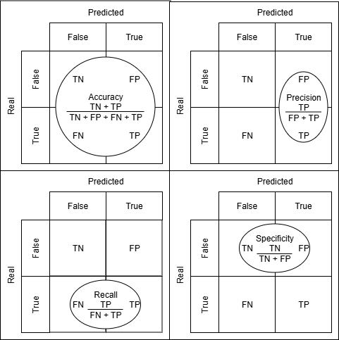 TP, TN, FP, FN for fraud detection. (Image: Hssiqueira, CC0, via Wikimedia Commons)
C. ROC Curve & AUC
- ROC Curve: Plots True Positive Rate (TPR) vs. False Positive Rate (FPR).
- AUC (Area Under Curve): 1 = perfect model, 0.5 = random guessing.
5. Feature Engineering & Hyperparameter Tuning
A. Feature Engineering
Improves model performance by:
- Scaling: Normalize features (e.g., Min-Max, StandardScaler) for algorithms like SVM.
- Encoding: Convert categorical data (e.g., "Male/Female" → 0/1 or one-hot encoding).
- Selection: Remove irrelevant features (e.g., using correlation analysis or PCA).
B. Hyperparameter Tuning
Algorithms have tunable parameters (e.g., max_depth in decision trees). Use:
- Grid Search: Exhaustive search over parameter combinations.
- Random Search: Faster alternative to grid search.
- Bayesian Optimization: Smart sampling of hyperparameters.
Example for Decision Trees:
from sklearn.tree import DecisionTreeClassifier
model = DecisionTreeClassifier(
    max_depth=5,          # Prevents overfitting
    min_samples_split=10, # Requires 10 samples to split
    criterion="gini"      # Splitting criterion
)
6. Real-World Applications in Nepal
A. Khalti: Fraud Detection
- Problem: Identify fraudulent transactions in real-time.
- Model: Random Forest Classifier (handles non-linearity, robust to outliers).
- Features: Transaction amount, time, location, user history.
- Output: Flag transactions with .
B. Daraz: Demand Forecasting
- Problem: Predict product demand to optimize inventory.
- Model: ARIMA (Time Series) for seasonal trends + Linear Regression for promotional effects.
- Features: Past sales, holidays, competitor prices.
- Impact: Reduces overstocking by 20%.
C. Pathao: Traffic Route Prediction
- Problem: Suggest fastest routes avoiding congestion.
- Model: Gradient Boosting (XGBoost) trained on GPS data.
- Features: Time of day, road conditions, historical traffic.
- Output: ETA with 90% accuracy.
7. Challenges & Best Practices
Common Pitfalls
- Overfitting: Model performs well on training data but poorly on unseen data.
- Solution: Use cross-validation, regularization, or simpler models.
- Data Leakage: Features from the future contaminate training (e.g., using next month’s sales to predict this month).
- Solution: Strict train-test splits, pipeline validation.
- Imbalanced Data: Rare events (e.g., fraud) dominate evaluation.
- Solution: Use SMOTE (synthetic oversampling) or F1-score over accuracy.
Best Practices
- Start simple: Begin with linear models before trying deep learning.
- Iterate: Use model pipelines (e.g., scikit-learn’s
Pipeline) to streamline workflows. - Explainability: For critical applications (e.g., loans), use SHAP values or LIME to interpret decisions.
Exam Tip
- Understand the difference between regression and classification—examiners often test this distinction.
- Memorize evaluation metrics (especially RMSE, precision/recall, AUC) and when to use each.
- Practical questions will ask you to:
- Interpret a confusion matrix or ROC curve.
- Choose the right algorithm for a scenario (e.g., "Which model for imbalanced data?" → SVM with class weights).
- Explain feature engineering steps (e.g., "How would you handle categorical variables?").
- Case studies may involve real-world data (e.g., "Predict NEPSE stock prices using ARIMA"). Practice with Kaggle datasets or local stock data.
- Diagrams are key: Be ready to sketch:
- A decision tree for a given dataset.
- A confusion matrix with TP/FP/FN/TN labels.
- A ROC curve with AUC interpretation.
Final Note: Predictive modelling is problem-driven. Master the algorithms, but focus on solving real problems—whether it’s optimizing Daraz’s inventory or detecting fraud in Khalti transactions. Use tools like Python (scikit-learn, XGBoost) or R (caret) to implement models and validate your understanding.
Based on the PU BE Computer (PU) syllabus for Data Science and Analytics (CMP422), unit 6.
Discussion
Loading…